Your prior is too informative?!

(Disclaimer: I perform a lot of frequency calculations in the post as approximations of Bayesian calculations.)

Suppose you have historical data that indicates a coin is biased. The data consists of \(100\) trials. From the data, we gathered that \(P_{Head} = 0.95\). We can use a normal approximation to justify that the Bernoulli parameter is somewhere between 0.906 and 0.994.

That’s a confidence interval of the form

\[ (l,u) = \left(\hat{p} - 2 \sqrt{\frac{\hat{p}(1-\hat{p})}{100}},\hat{p} + 2 \sqrt{\frac{\hat{p}(1-\hat{p})}{100}}\right). \]

Your company is getting ready to buy a brand new coin, and one of the main requirements is that the new coin has to be biased with \(P_{Head}\) at least \(0.80\). The new coin is similar to the old coin, but it’s brand new from the treasury, which has recently changed its minting process. The treasury says everything about the new coin is better than the old one: It’s shinier, lighter, more durable, and just as reliable as the old coin, despite the new materials.

Unfortunately, testing the new coin is costly, we’ll only get a few trials to infer its bias. The historical data was collected over the course of several years, and is considered pretty good stuff, so we are asked if we can apply some Bayesian techniques to use the old data to say something about how many trials we need to do to test the bias of the new coin.

Now here’s two identical ways to reuse the historical data:

1. (Frequentist perspective) Reusing the historical coin flips is the same as pooling the old and new coin flips together

2. (Bayesian perspective) The prior for the new experiment is exactly the posterior from the old experiment (which I approximated above with the interval \((l,u)\)).

(Of course, the other easy option is completely rejecting the historical data.)

The Bayesian method implies that the exact posterior from the historical data should be treated as the prior distribution for analysis of the upcoming experimental data. This is seductive because it bypasses the need to interrogate the prior distribution, but the idea that new and old data are exchangeable is highly suspect. Often, statisticians do not consider this dangerous implication.

In reality, the ‘correct’ prior distribution is not the posterior from the previous test, because we don’t know that the new coin will be similarly biased like the old coin (with high confidence). It’s our job to determine that! This is assuming the conclusion. The correct prior is somewhere between the posterior of the historical data and complete ignorance of the historical data, which lands us squarely back in subjective Bayesian analysis.

If we assume exchangeability of old and new data, we are (maybe?) implicitly saying that we don’t need to do any testing at all: Suppose we can plan to execute \(5\) flips of the new coin, and all flips end up as tails (worse case scenario). Now the new+old estimate of \(P_{Head}\) is \(95/105 =\) 0.905, and the new+old confidence interval for the coin bias is 0.846 to 0.963.

So even if the new coin utterly fails the test, we can still say, with high confidence, that the bias of the coin exceeds \(80\%\). Might as well not test at all in this situation!

For this unfortunate reason, in this case we could resort to a ‘dual prior’ solution: a non-informative design prior, and an informative analysis prior. But this is just hogwash– we’re just picking and choosing to use an informative prior when it’s convenient and otherwise ignoring it.

One solution to the “prior data is too informative” predicament is to actually get serious about prior distributions: We don’t seriously think the posterior from the old experiment summarizes our prior state of knowledge of the bias parameter of the new coin. It’s just information that guides determination of a better prior.¹ It is perhaps reasonable to put the mode of the prior distribution at \(P_{Head}^{Old}=0.95\), but we should not let the old posterior variance determine the prior variance.

In this case, we need to consider how far astray \(P_{Head}^{New}\) could drift from old data, and set a prior variance that summarizes this belief. It’s entirely possible that \(P_{Head}^{New}\) could be (say) \(10\%\) lower. In this case I might follow the Stan manual and recommend a truncated Normal distribution, or something similar.².

This is very similar to making a statement about the value of old data. Is one old data point worth the same as one new data point? Is it worth half as much? The value ratio of old to new is the same as the prior variance of the coin’s bias parameter. In my case, maybe a truncated Normal distribution with mean \(0.95\) and standard deviation \(0.10\) summarizes the value of the historical coin data. This is wide enough that the new data has enough punch to surprise me.

A graph of my prior:

library(ggplot2)

x <- rnorm(10000, 0.95, 0.1)
x <- x[x > 0 & x < 1] #truncate the normal to [0,1]

theme_set(theme_bw(base_size = 16))

ggplot(data.frame(x = x), aes(x = x)) +
  geom_histogram(fill = "royalblue2", color = "black", bins = 30) +
  xlab("Samples from my truncated Normal prior") +
  ylab("") +
  geom_vline(aes(xintercept = 0.95), size = 1.5) # prior mode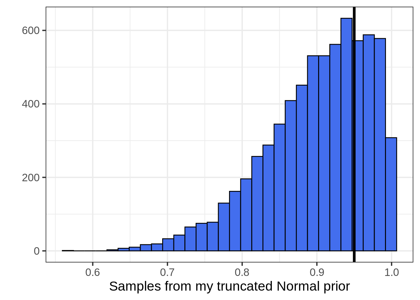

One way to think about my prior is that, given the historical coin flips, I think the new coin will exceed the point 0.80 threshold with probability 0.903.

Takeaway: Getting serious about data reuse means we have to think hard about the value of old data. Data ages like milk. We need to dilute the value of old data in order to learn from it. This dilution is subjective, but beats the other ends of the spectrum (complete data pooling and complete rejection of old data).