Simulate some fake data

dat <- gamSim(4, n = 400, dist = "normal", scale = 1)

## Factor `by' variable example

The simulation creates a dataframe with a single response and 3 numeric covariates. The effect of each covariate depends on the value of a factor, fac.

We can take a look at the data by plotting the response against each of the covariates:

ggplot(dat, aes(x = f1, y = y)) +
  geom_point(size = 1.5) +
  ggtitle("y versus f1:") +
  facet_wrap( ~ fac)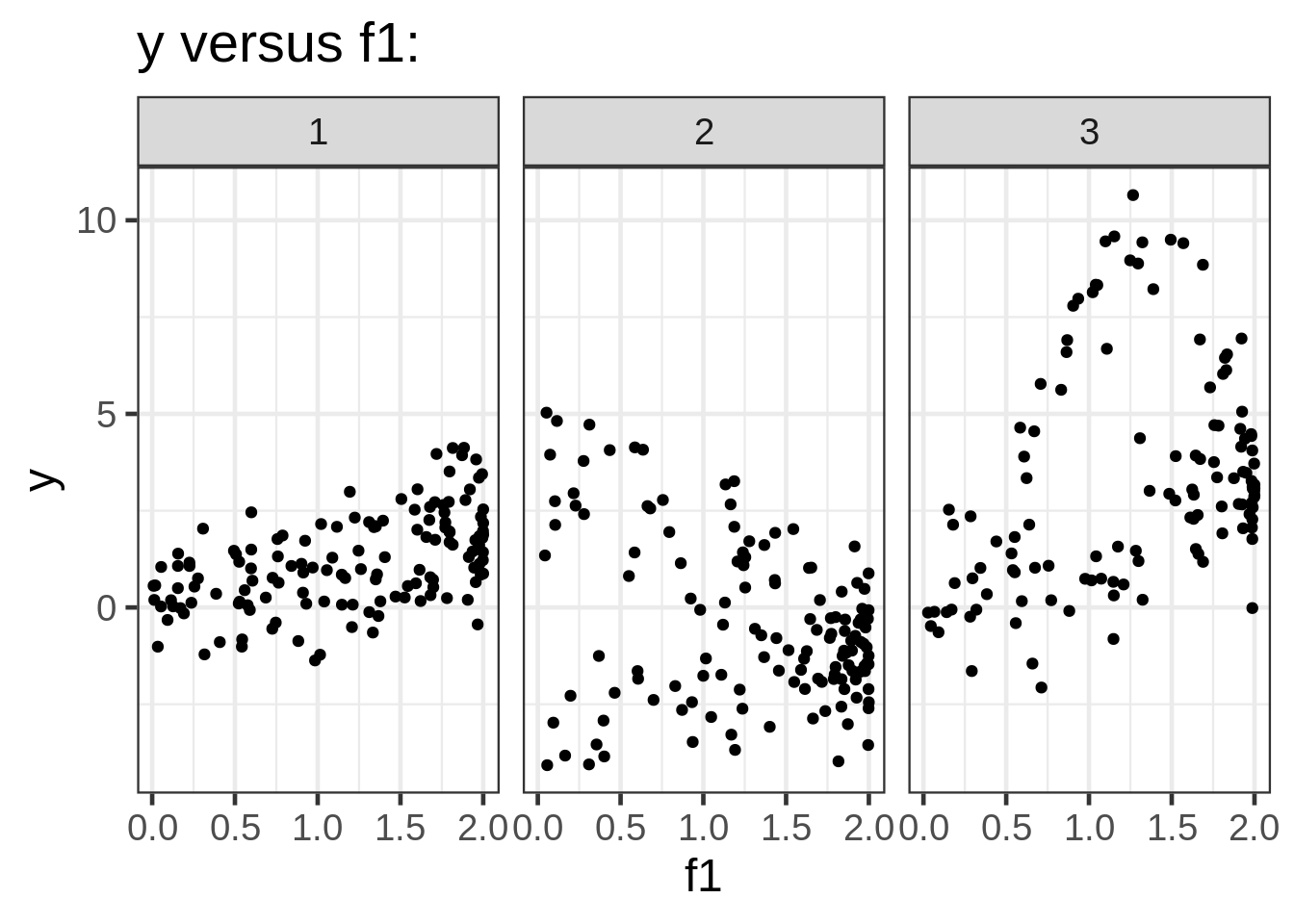

ggplot(dat, aes(x = f2, y = y)) +
  geom_point(size = 1.5) +
  ggtitle("y versus f2:") +
  facet_wrap( ~ fac)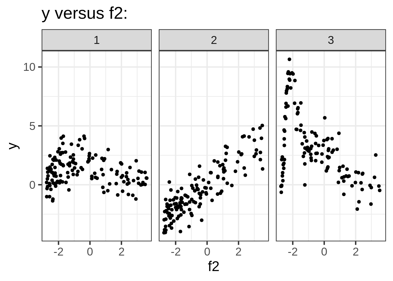

ggplot(dat, aes(x = f3, y = y)) +
  geom_point(size = 1.5) +
  ggtitle("y versus f3:") +
  facet_wrap( ~ fac)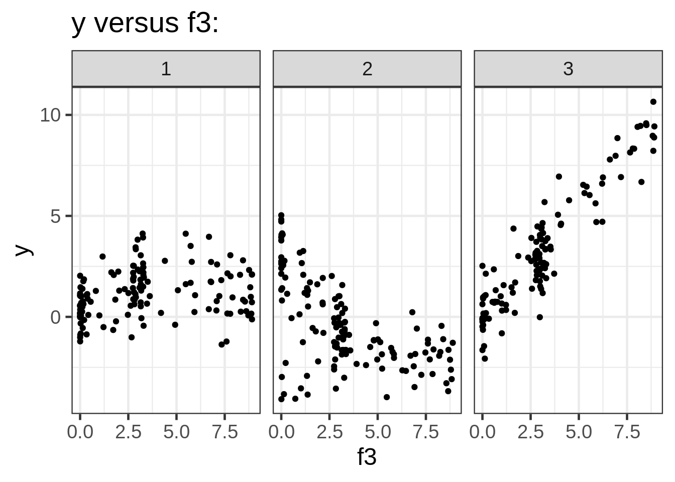

Separate Smoothers

The usual way to fit the data in mgcv is to use the by argument. This results in a different smooth for each level of the factor. Ie, the smoothing parameters for each of the continuous factors is allowed to vary with each level of fac. Now, we can get really fancy here by changing the knots, smoothers, adding interactions, model checking, yada yada, but I just want a model fit to compare apples-to-apples with the other method.

fit1 <- gam(y ~ fac + s(f1, by = fac) + s(f2, by = fac) + s(f3, by = fac), data = dat)
dat$preds1 <- predict(fit1)

A summary of the model fit shows that separate smooths are created for each numeric covariate and each level of fac:

summary(fit1)

## 
## Family: gaussian 
## Link function: identity 
## 
## Formula:
## y ~ fac + s(f1, by = fac) + s(f2, by = fac) + s(f3, by = fac)
## 
## Parametric coefficients:
##             Estimate Std. Error t value Pr(>|t|)    
## (Intercept)  1.23062    0.08879   13.86   <2e-16 ***
## fac2        -1.69374    0.12581  -13.46   <2e-16 ***
## fac3         2.21761    0.12962   17.11   <2e-16 ***
## ---
## Signif. codes:  0 '***' 0.001 '**' 0.01 '*' 0.05 '.' 0.1 ' ' 1
## 
## Approximate significance of smooth terms:
##              edf Ref.df       F  p-value    
## s(f1):fac1 1.703  2.129  19.367 4.83e-09 ***
## s(f1):fac2 1.629  2.019   0.767    0.490    
## s(f1):fac3 1.000  1.000   0.274    0.601    
## s(f2):fac1 1.000  1.000   0.003    0.957    
## s(f2):fac2 1.000  1.000 233.375  < 2e-16 ***
## s(f2):fac3 1.000  1.000   0.048    0.827    
## s(f3):fac1 1.000  1.000   0.009    0.925    
## s(f3):fac2 1.000  1.000   0.939    0.333    
## s(f3):fac3 1.000  1.000 435.018  < 2e-16 ***
## ---
## Signif. codes:  0 '***' 0.001 '**' 0.01 '*' 0.05 '.' 0.1 ' ' 1
## 
## R-sq.(adj) =  0.843   Deviance explained = 84.8%
## GCV = 1.1138  Scale est. = 1.0767    n = 400

ggplot(dat, aes(x = f1, y = y)) +
  geom_point(size = 1.5) +
  geom_line(aes(y = preds1), size=1.5, color = "blue") +
  facet_wrap( ~ fac)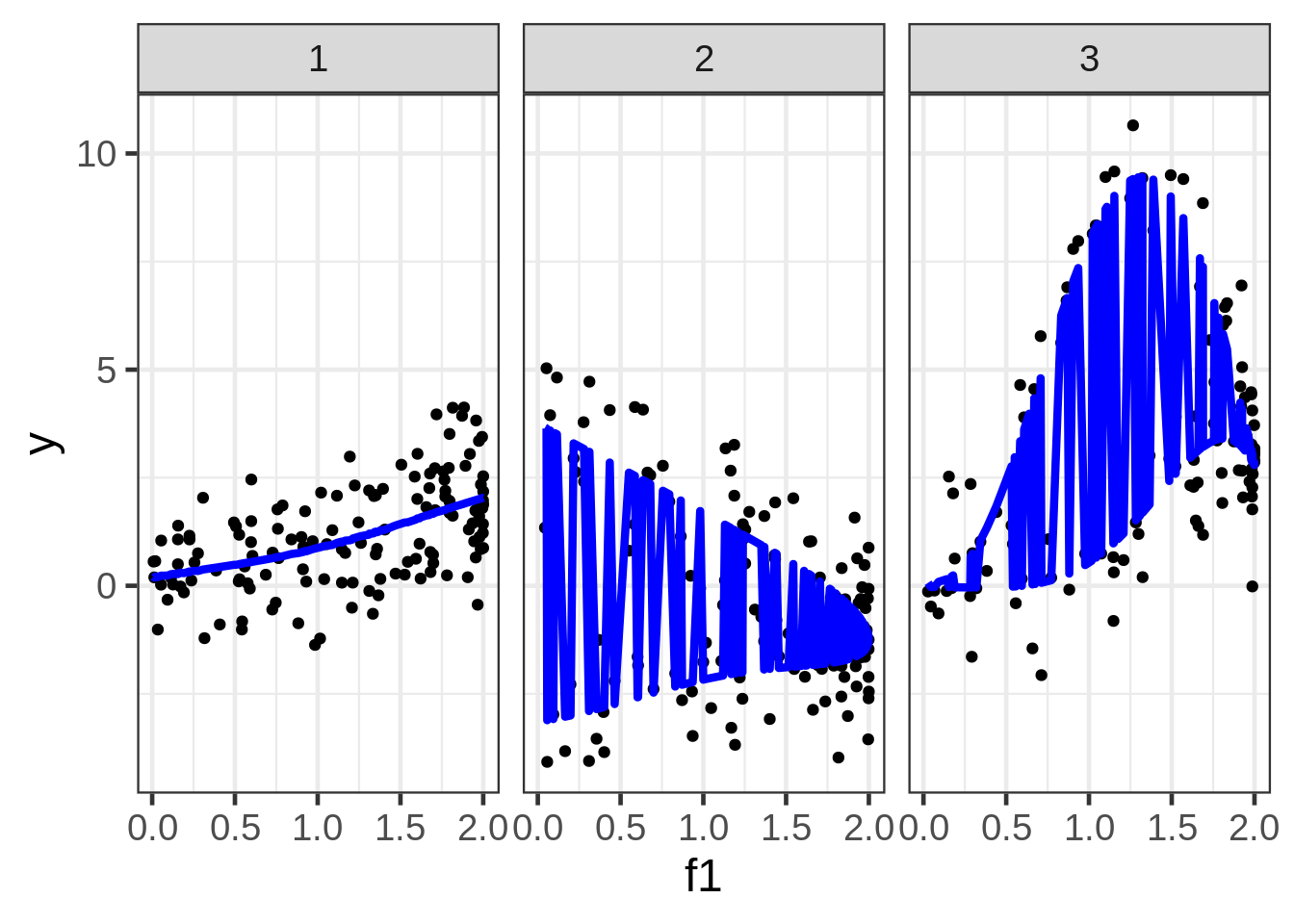

We can plot the predictions, but the picture is very poor because the preds also depend on f1 and f2, which are not shown, and are varying behind the scenes. Although this gives us some nice information about the extent that \(E(y)\) could vary as a function of all three covariates, it’s almost certainly not the plot we want to draw. A solution is to fix f2 and f3 at some representative values.

new <- data.frame(
  f1 = dat$f1,
  fac = dat$fac,
  f2 = median(dat$f2),
  f3 = median(dat$f3))

dat$preds1_f1 <- predict(fit1, newdata = new)

ggplot(dat, aes(x = f1, y = y)) +
  geom_point(size = 1.5) +
  geom_line(aes(y = preds1_f1), size=1.5, color = "blue") +
  facet_wrap( ~ fac)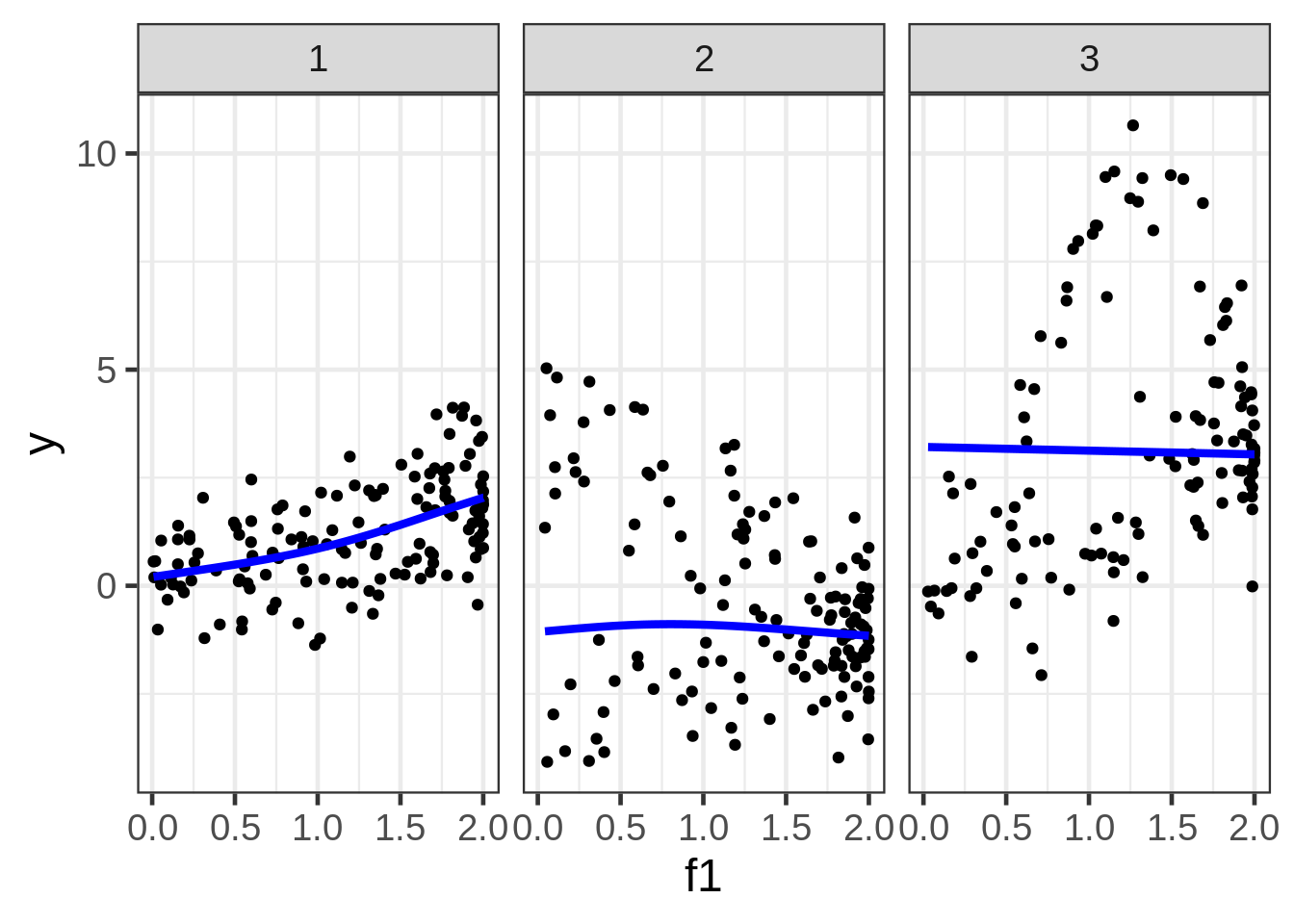

Well, the resulting marginal¹ smooths are not very exciting. The smooth for second facet looks particularly misleading, but I don’t see a way around that when we are in the business of making a 2D plot of what is a 5D relationship.

Sharing the smoothing parameter

An alternative is to create smooths which share the same smoothing parameter over the level of fac. Mgcv provides this capability through bs="fs"

fit2 <- gam(y ~ fac + s(f1, fac, bs = "fs") +
              s(f2, fac, bs = "fs") +
              s(f3, fac, bs = "fs"), data = dat)

## Warning in gam.side(sm, X, tol = .Machine$double.eps^0.5): model has repeated 1-
## d smooths of same variable.

dat$preds2_f1 <- predict(fit2, new)

A summary of the model fit shows that the same smoothing parameter is used for each numeric covariate, regardless of the factor levels of fac.

summary(fit2)

## 
## Family: gaussian 
## Link function: identity 
## 
## Formula:
## y ~ fac + s(f1, fac, bs = "fs") + s(f2, fac, bs = "fs") + s(f3, 
##     fac, bs = "fs")
## 
## Parametric coefficients:
##             Estimate Std. Error t value Pr(>|t|)  
## (Intercept)   0.9375     0.7201   1.302   0.1937  
## fac2         -1.2106     1.0191  -1.188   0.2356  
## fac3          2.4397     1.0191   2.394   0.0171 *
## ---
## Signif. codes:  0 '***' 0.001 '**' 0.01 '*' 0.05 '.' 0.1 ' ' 1
## 
## Approximate significance of smooth terms:
##             edf Ref.df      F  p-value    
## s(f1,fac) 4.000     28  1.378 4.32e-09 ***
## s(f2,fac) 2.953     27  8.619  < 2e-16 ***
## s(f3,fac) 3.000     28 13.804  < 2e-16 ***
## ---
## Signif. codes:  0 '***' 0.001 '**' 0.01 '*' 0.05 '.' 0.1 ' ' 1
## 
## R-sq.(adj) =  0.843   Deviance explained = 84.8%
## GCV = 1.1133  Scale est. = 1.0773    n = 400

Again, we can take the marginal predictions and plot them against the data. This time, we plot the new preds in red to see if there is a difference.

ggplot(dat, aes(x = f1, y = y)) +
  geom_point(size = 1.5) +
  geom_line(aes(y = preds1_f1), size=1.5, color = "blue") +
  geom_line(aes(y = preds2_f1), size=1.5, color = "red") +
  facet_wrap( ~ fac)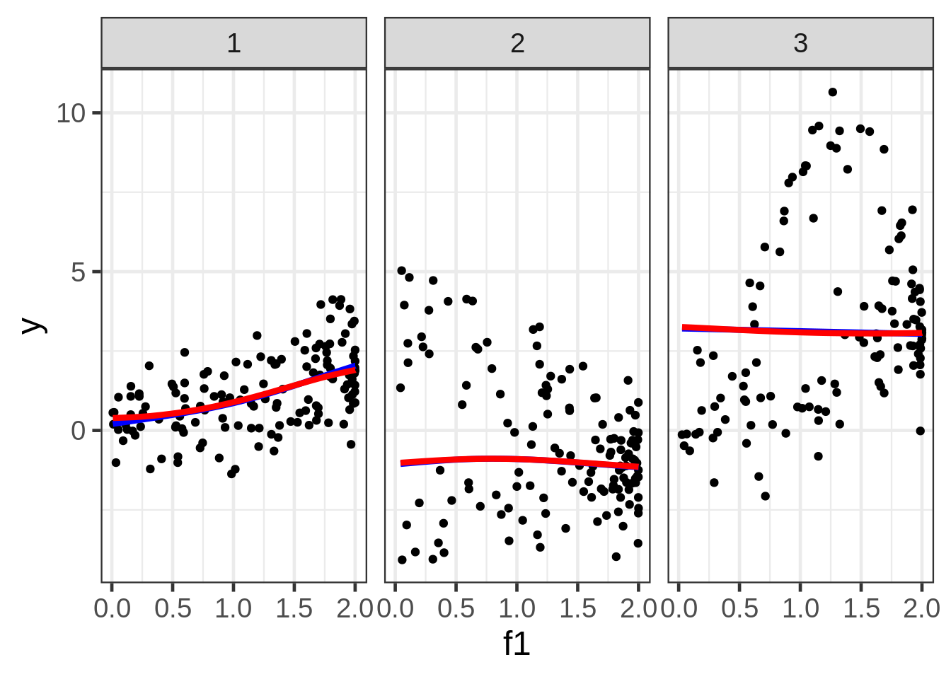

There is no great difference in our simple example between the two types of fits. I suppose this is because we have a very small number of groups; not enough to show the advantages and differences between the two fits. According to the mgcv docs, bs="fs" is useful when we have many groups, and there is a need to reuse the same smoothing parameter across all groups – a strange kind of homogeneity, if you ask me.

I’m not able to find anything in Simon Wood’s GAM book about ‘fs’ smooths, which leads me to think they are a recent addition to the mgcv package. For more information on smoothing with respect to groups in mgcv, the help page for smooth.construct.fs.smooth.spec is useful.

To end the post, it’s worth taking a look at the marginal plots of the other two factors to see if there are some differences.

new2 <- data.frame(
  f1 = median(dat$f1),
  fac = dat$fac,
  f2 = dat$f2,
  f3 = median(dat$f3))

new3 <- data.frame(
  f1 = median(dat$f1),
  fac = dat$fac,
  f2 = median(dat$f2),
  f3 = dat$f3)

dat$preds1_f2 <- predict(fit1, newdata = new2)
dat$preds2_f2 <- predict(fit2, newdata = new2)

dat$preds1_f3 <- predict(fit1, newdata = new3)
dat$preds2_f3 <- predict(fit2, newdata = new3)

ggplot(dat, aes(x = f2, y = y)) +
  geom_point(size = 1.5) +
  geom_line(aes(y = preds1_f2), size=1.5, color = "blue") +
  geom_line(aes(y = preds2_f2), size=1.5, color = "red") +
  facet_wrap( ~ fac)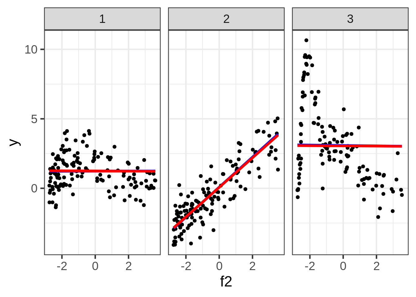

ggplot(dat, aes(x = f3, y = y)) +
  geom_point(size = 1.5) +
  geom_line(aes(y = preds1_f3), size=1.5, color = "blue") +
  geom_line(aes(y = preds2_f3), size=1.5, color = "red") +
  facet_wrap( ~ fac)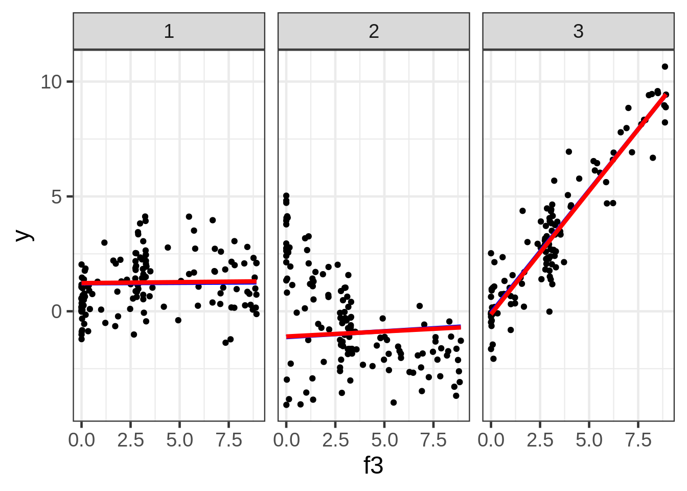

Again, no huge difference between the two fitting strategies. But the poor marginal fits shows the danger of looking at complicated, multivariate models from a 2D view.