Bayesian Power
Power is an idea from frequency statistics that is used by some to judge the quality of an experimental design. I don’t think power is (or should be) a universal design requirement, but it seems to get into just about any design – even experiments that do not intend to analyze data using ANOVA, or something like that. Briefly, for a simple test of \(H_0\) vs \(H_1\),
\[ \textrm{Power} = \textrm{Pr}(\textrm{Reject Null} | \mathrm{H_1}) \]
We typically strive to have experiments with large power, but the dependece on \(H_1\), the confidence level, prior study variability, make power tricky and easy to misuse. However, for reliability/survival experiments power can take a different, simpler form. In this post, we explore that form, and display some different versions.
Notably, we will discuss a Bayesian version of power. There are many Bayesian analogs to power, but the one used in this note is
\[ \textrm{Power} = \textrm{Pr}_{\mathcal{X}} (\textrm{Pr}_{\Theta|x}(\theta \in R)). \]
where \(\mathcal{X}\) is the sample space of the data, \(\mathcal{\Theta}\) is the support of the parameter \(\theta\), and \(R\) is the region where we would like to observe \(\theta\). In english, this version of Bayesian Power is the probability is obtaining a posterior probability that is suitably large.
This is one of those weird Bayesian situations where integration over the sample space seems like a good idea, but this is only because we’ve yet to observe any data at all.
Intro
Many units have a reliability requirement. For example, a car must be at least 80% reliable – this means that the probability of failure during a trip is less than or equal to 20%. (Yes, this reliability is very low for a car, just an example!) In testing the car, since we typically size a test to have at least 80% power, it is natural to find the test that has at least 80% probability that the requirement is met (that the reliability is at least 80%).
Conditional (classical) power w/ flat prior
Suppose we conduct a test of 12 trips, and observe 3 failures. A failure is like a Bernoulli outcome, either the unit failed or it did not. The likelihood for reliability is \(\propto p^{9} (1-p)^3\). Using a flat prior, we can treat the likelihood as a posterior probability density and say that there is a
\[ \frac{\int_{0.8}^1 p^9 (1-p)^3 dp}{\int_0^1 p^9 (1-p)^3 dp} \]
probability of meeting the requirement, given the observed data. Numerically, There is a
like = function(p, r) ( p ^ r ) * ( (1 - p) ^ (12 - r) ) # p is the prob of not failing, and r is the number of successful missions.
integrate(like, 0.8, 1, r = 9)$value / integrate(like, 0, 1, r = 9)$value
## [1] 0.2526757probability of meeting the requirement. So, while 9/12 is pretty close to 0.8, the actually probability of meeting/exceeding the reliability threshold given test outcomes is low.
Note: We are lucky here to be able to say that “there is a 25% chance of meeting the requirement” because it’s not controversial to use a uniform prior for the Bernoulli likelihood AND because the hypothesis test
\[ H_0 : \textrm{Reliability} < 0.8\\ H_1 : \textrm{Reliability} > 0.8 \]
is more sensible than something like
\[ H_0 : \textrm{Reliability} = 0.6\\ H_1 : \textrm{Reliability} = 0.9 \]
Borrow information from a previous test
Suppose last year’s car had 10 failures in 80 trips, so we might estimate that its reliability is about 88%. The new car is planning on 12 trips to complete its round of testing. Is that enough?
Suppose we believe the new car’s reliability is also something like 88%. Then we can determine the ‘power’ of the test to assess reliability via simulation.
Reliability Power assuming flat prior, conditional on one alternative.
We need to do a simulation, because we don’t know for sure what to expect from the data:
nsim <- 1000


prob_meet_requirement <- success <- rep(NA, nsim)

for(i in 1:nsim) {
  success[i] <- rbinom(1, 12, 0.88)
  prob_meet_requirement[i] <- integrate(like, 0.8, 1, r = success[i])$value / integrate(like, 0, 1, r = success[i])$value
}

mean(prob_meet_requirement) #power
## [1] 0.6464293The expected power of the test (conditional on the \(\textrm{Binomial}(p=0.88, n=12)\) distribution) is unfortunately too low to let us say the size of the test is large enough to meet the reliability requirement with confidence.
Conditional Power w/ Informative Prior
We could have conducted the Bayesian power analysis using a more informative prior distribution. Last year’s car model had a reliability of \(0.88\). We think this year’s car will have a similar reliability, but since the data is a bit old at this point, the posterior standard error of last year’s analysis is perhaps not the most applicable. We will cautiously assume the new car’s reliability might be like a normal distribution, centered at mean \(0.88\) and standard deviation \(0.1\). However, since probabilities are between 0 and 1, we truncate the normal distribution to have support \([0,1]\).
It is nice to take a look at the prior distribution before the analysis:
library(ggplot2)
library(truncnorm)
theme_set(theme_classic(base_size = 18))

ggplot(data.frame(x = c(0, 1)), aes(x = x)) +
  stat_function(fun = "dtruncnorm", args = list(a = 0, b = 1, mean = 0.88, sd = 0.1)) +
  geom_vline(aes(xintercept = 0.8), linetype = "dotted") +
  xlab('Reliability') +
  ylab('Density') +
  ggtitle("Our Prior")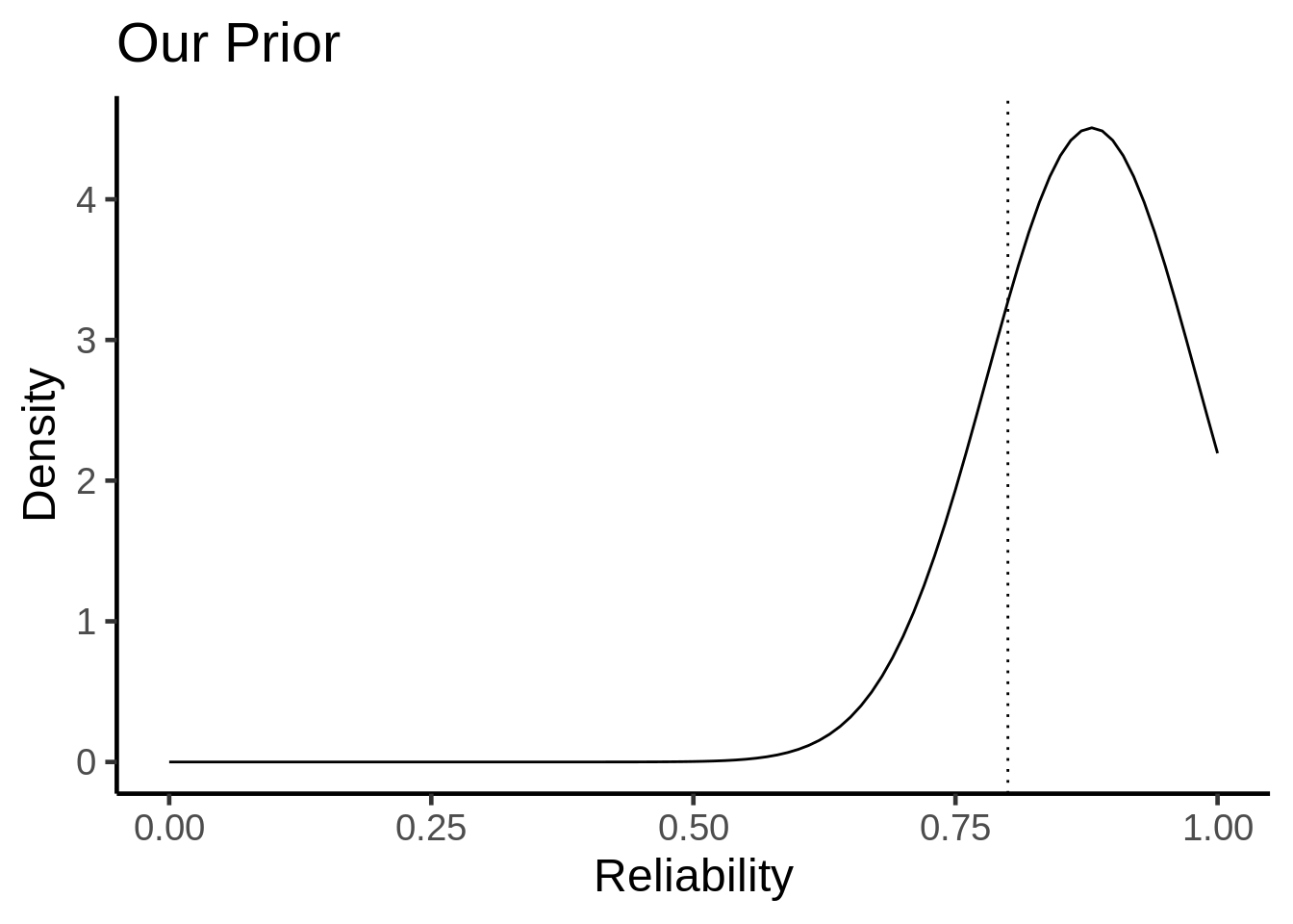
Define a function that is proportional to the posterior distribution:
prop_to_post <- function(p, r) {
  like(p, r) * dtruncnorm(p, 0, 1, 0.88, 0.1) # proportional to likelihood times prior.
}
Now, given a set of successes, the probability of exceeding the reliability threshold of 0.8 is given by
\[ \frac{\int_{0.8}^1 p^r (1-p)^{n-r} \pi (p) dp}{\int_0^1 p^r (1-p)^{n-r} \pi (p) dp} \]
where the likelihood is the same as before and \(\pi\) is the truncated normal prior.
nsim <- 1000

prob_meet_requirement <- success <- rep(NA, nsim)

for(i in 1:nsim) {
  success[i] <- rbinom(1, 12, 0.88)
  prob_meet_requirement[i] <- integrate(prop_to_post, 0.8, 1, r = success[i])$value / integrate(prop_to_post, 0, 1, r = success[i])$value
}

mean(prob_meet_requirement) #power
## [1] 0.8115299And of course, the “power” is higher because we used an informative prior that is biased in favor of meeting the threshold. Under this prior distribution, the size of the test may be adequate.
Unconditional Power w/ Informative Prior
There is one more aspect of Bayesian Power to document. That is the situation where we do not condition on a specific alternative hypothesis. I will call this ‘unconditional power’, because I intend to integrate the distribution of power over a set of possible alternative hypotheses, thus incorporating my possible uncertainty in how to conduct the power analysis.
The only change is that instead of generating data under a specific alternative hypothesis, \(y|p=0.88 \sim \textrm{Binomial}(12, 0.88)\), I will generate data from the compound distribution
\[ y|p \sim \textrm{Binomial}(12, p)\\ p \sim \textrm{Truncated Normal}_{[0,1]}(0.88, 0.05) \]
This is a straight-forward adjustment to the power calculation from before.
I will update the calculation with the truncated normal prior, but we can similarly update the calculation with the non-informative prior. In my opinion this ‘unconditional power’ could be more honest that power conditional on a single alternative hypothesis, but in practice this could depend heavily on the alternative distribution.
Here is my simulation, which uses an informative prior distribution and a jittery alternative distribution:
nsim <- 1000

prob_meet_requirement <- success <- rep(NA, nsim)

for(i in 1:nsim) {
  p_alt <- rtruncnorm(1, 0, 1, 0.88, 0.1)
  success[i] <- rbinom(1, 12, p_alt)
  prob_meet_requirement[i] <- integrate(prop_to_post, 0.8, 1, r = success[i])$value / integrate(prop_to_post, 0, 1, r = success[i])$value
}

mean(prob_meet_requirement) #power
## [1] 0.7634455Note that
1 - ptruncnorm(0.8, 0, 1, 0.88, 0.05)## [1] 0.9447478is the amount of probability in the region of the alternative distribution – so this is an upper bound for unconditional Bayesian power in this set up.