The effect of imbalance on power in the two-sample proportions test

Generally, data imbalance is thought to be bad in experiments, but this is not always the case. Suppose you want to study the effect of a drug on \(Pr(Survival)\). In a trial where the cost of enrolling a subject for the treatment or control is identical, then the optimal experiment (from the statistician’s perspective) is to roughly balance the treatment and control groups.

This is the assumption power.prop.test makes in R when it calculates the power of a two-sample proportions test.

However, in many experiments the treatment is an expensive intervention, and there is no placebo that we could give to the control subjects. In this case the study groups are ‘received intervention’ (treatment) and ‘did not receive intervention’ (control). In these experiments, the cost of control is negligible compared to the cost of treatment, so this should factor into the experimental design. So what is the effect on power?

Suppose first that we have equal group sizes. Then we can use the built-in R function:

power.prop.test(200, 0.5, 0.6)

## 
##      Two-sample comparison of proportions power calculation 
## 
##               n = 200
##              p1 = 0.5
##              p2 = 0.6
##       sig.level = 0.05
##           power = 0.5200849
##     alternative = two.sided
## 
## NOTE: n is number in *each* group

So a total sample size of 400 is needed to study a 10% effect size to get about 50% power. It’s important that the effect is a difference between 60% and 50% because effects near 50% are the noisiest (hardest to study).

Now consider the case where the control group can be much larger than the treatment group. Let’s again take the treatment group to be 200 subjects, and let the control group increase in size. Then the power of the test should increase – but not approach 1.

We can test the hypothesis with a simulation. As mentioned earlier, R has no built-in test for the unbalanced two sample problem, so we can write our own, or use a function from the pwr library. I will write my own.

# get the power for two groups with different probs and different sample sizes:
# use logistic regression parameterization
get_power_2p2n <- function(nsim, p1, p2, n1, n2){

  p <- rep(NA, nsim)

  for(i in 1:nsim){
    s1 <- rbinom(n1, 1, p1)
    s2 <- rbinom(n2, 1, p2)
    dat <- data.frame(y = c(s1, s2),
                      g = c(rep("g1", n1), rep("g2", n2)))
    fit <- glm(y ~ g, data = dat, family = binomial)
    p[i] <- summary(fit)$coefficients[8]
  }

  mean(p < 0.05)
}

Here’s a quick check that the function is approximately correct compared to the well-tested power.prop.test:

get_power_2p2n(1000, 0.5, 0.6, 200, 200)

## [1] 0.51

Since the power is just about 50%, I think we can go ahead and use it.

Now for the simulation. We apply the function to a range of sample sizes of the control group. We start with 200 subjects and increase up to 1000.

p1 = 0.5
p2 = 0.6
nsim = 2500
ntreat = 200
ncontrol = ntreat * seq(1, 5, by = 0.5)

out <- rep(NA, length(ncontrol))

for (i in 1:length(ncontrol)) {
  out[i] <- get_power_2p2n(nsim, p1, p2, ncontrol[i], ntreat)
}

pdat <- data.frame(control_size = ncontrol,
                   power = out)

library(ggplot2)
theme_set(theme_bw(base_size = 16))

ggplot(pdat, aes(x = control_size, y = power)) +
  geom_point(size = 2) +
  geom_line() +
  xlab('control group size') +
  ggtitle("Power as control group size increases", "Treatment group size fixed at 200")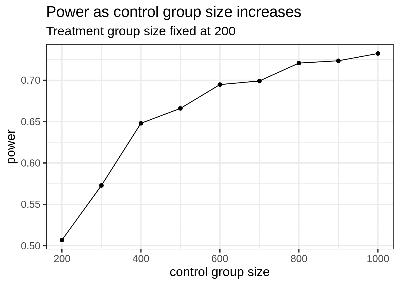

Somewhat expected, the power does increase, but the gains level off. By increasing control group size, we might see modest increases in power, but not nearly the same as if we increased the size of both groups together. Even when the control group is 5 times bigger than the treatment group, we can only get the power to increase from 50% to 75%.

Here’s what it looks like if you increase both groups. This sim is much easier because we can use the built-in R function.

p1 = 0.5
p2 = 0.6
nsim = 2500
ntreat = 200
ncontrol = ntreat * seq(1, 5, by = 0.5)

out <- power.prop.test(ncontrol, p1, p2)$power

pdat <- data.frame(control_size = ncontrol,
                   power = out)

ggplot(pdat, aes(x = control_size, y = power)) +
  geom_point(size = 2) +
  geom_line() +
  xlab('control/treatment group size') +
  ggtitle("Power as control AND treatment group\nsizes increase together")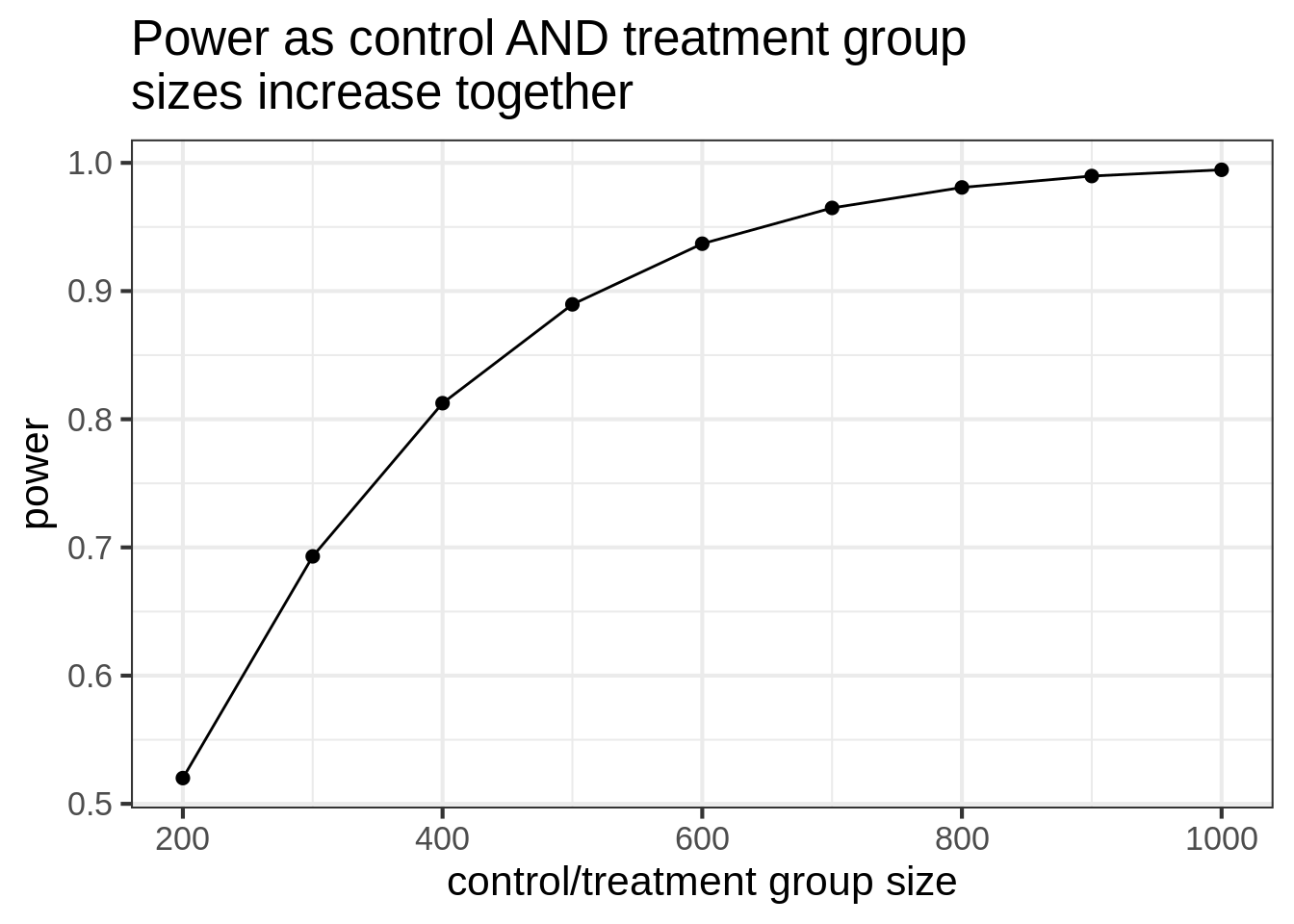

Notice that when we increase the control group size while fixing treatment size at 200, the power tops out at 75%. But in the balanced simulation, the power hits 80% when both groups are size 400.

So, if it’s easy to collect a lot of (good) control group data, you do see increases in power, but it’s not nearly as good as getting an equal amount of data on both groups.