Despite the spartan looks of this website, it is actually a low-key Javascript monster. I’m not really sure how this happened, but I don’t know a lot about websites, and I just kind of trust that if I don’t do too much fiddling then the website will be fast.
I’m disappointed to find that it takes several seconds to load most of the pages on randomeffect.net. I’m trying to use Chrome’s devtools to figure out the culprits, and I think I have it narrowed down to either the syntax highlighting JS or the comments section JS. Which is a shame because both of these features seem to be pretty necessary for a good blog about statistics.
But I know the importance of having a fast website. No one likes to wait a couple seconds for a page to load. Luckily the main text on all the pages loads almost instantly while the less important elements take some extra time.
To make a decision about which features to remove from the website, we need to conduct a small experiment. Based on the results of the experiment and my personal utility functions, I can make a decision about which (if any) features should be removed.
How this site is hosted
Following the advice the blogdown book, I registered a domain with Google Domains and host the website with Netlify (free tier). I don’t think there is any throttling from Netlify, but I only skimmed their terms of service.
I access the website from my home internet connection, some middle-of-the-road connection from Comcast and view the website on a 2015 laptop running Ubuntu.
Possible Culprits
Here are the tweaks I made to the xmin hugo theme that could have caused the website to slow down:
- What I want to test:
- Added Disqus comments
- Added syntax highlighting
- Tweaks I made that may only have minimal performance impact
- Added table of contents to some pages
- Added links in the footer that let users jump to next/previous post
- Added pagination to the home page
- Displayed categories and tags to each of the blog posts
Perhaps notable, I have never put Google Analytics on the blog.
A profile in Chrome
I use Firefox, but everyone says the Chrome has better devtools, so we’ll use Chrome for the profiling. Let’s open up a post and see how long it takes. Right now I have highlighting disabled and comments on. Here is what Lighthouse has to say about my homepage:
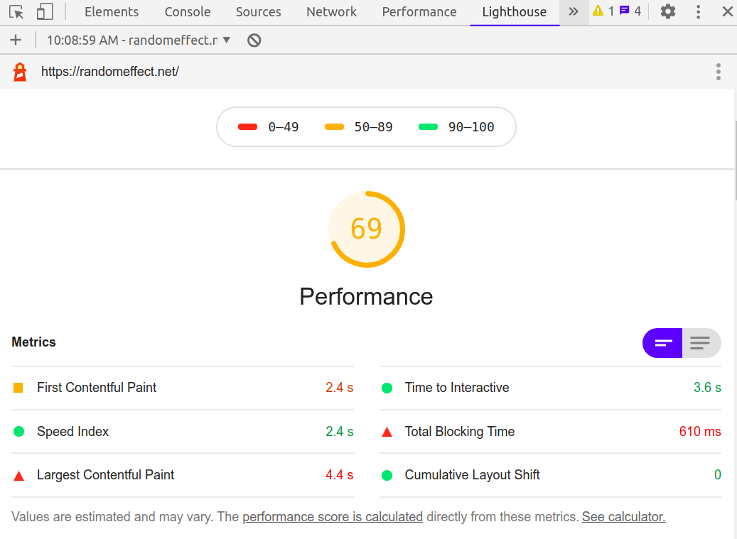
Lighthouse says my page is slow. When I open up the network profiler, the page takes between 0.5 and 1 second to load. I opened my page on estimating interaction powers and found that it takes 7 seconds to load! Unacceptable!
How do JS elements affect load time?
The model for the page load times is
\[ \mathrm{load time} = \beta_0 + \beta_1 \times 1_{\mathrm{Comments On}} + \beta_2 \times 1_{\mathrm{Syntax HL On}} + \beta_3 \times 1_{\mathrm{Both On}} + \varepsilon, \]
where \(\varepsilon\) is a Normal deviate, and the \(\beta\)’s are the effect of each the JS elements in the experiment. So I think about load times as a linear model, which will be helpful to determine if the effects of comments and syntax highlighting are significant. This is a bit overkill, but lets me flex my statistical muscles and make up for the fact that I don’t understand Chrome’s page profiler very well.
I think the Normal assumption is probably a good one: it makes sense that load times would be roughly symmetric around a value if we test the website from the same internet connection.
If the load times are right skewed, a log-normal model could make more sense.
How much data?
We are lucky because the data doesn’t take much time and money to collect, so a power analysis is unnecessary. I will collect \(10\) load times per stratum from the same webpage and use an orthogonal experimental design (full factorial).
Experimental Data
I will collect \(40\) load times according to the two-way table defined by Syntax on (Yes/No) and Comments on (Yes/No). The data are:
dat <- data.frame(
  hl_off_comments_off = c(1.27, 0.56, 0.55, 0.75, 0.46, 0.53, 0.51, 0.54, 0.48, 0.55),
  hl_off_comments_on = c(5.62, 4.39, 4.39, 4.99, 4.31, 4.38, 4.61, 5.55, 4.05, 4.25),
  hl_on_comments_off = c(2.47, 0.99, 1.01, 1.47, 1.12, 1.88, 1.77, 0.89, 1.09, 1.36),
  hl_on_comments_on = c(7.52, 5.69, 5.14, 5.79, 5.58, 6.03, 5.70, 5.41, 6.76, 6.47)
)
Measurements of load time are taken in seconds using the Chromium web browser with network cache disabled. The data are not ‘tidy’ so we need to fix that.
Inspect the data
The first thing is always… visualize the data! We use ggplot2. We need to clean the data. I’m not so good with the tidyverse one-liners, so please excuse my brute-force method:
library(ggplot2)
library(tidyr)
library(RColorBrewer)
theme_set(theme_bw(base_size = 18))

## make data tidy
dat <- gather(dat)
dat$comments <- grepl("comments_on", dat$key)
dat$syntax_hl <- grepl("hl_on", dat$key)
dat$loadtime <- dat$value
dat <- dplyr::select(dat, -c(key, value))

head(dat)
## comments syntax_hl loadtime
## 1 FALSE FALSE 1.27
## 2 FALSE FALSE 0.56
## 3 FALSE FALSE 0.55
## 4 FALSE FALSE 0.75
## 5 FALSE FALSE 0.46
## 6 FALSE FALSE 0.53ahh, that’s what I want :)
Now we can plot it:
ggplot(dat, aes(x = comments, y = loadtime, group = syntax_hl, color = syntax_hl)) +
  ggtitle("Webpage load times",
          "Factorial experiment results\n(two factors: syntax highlighting and comments)") +
  scale_color_brewer(palette = "Set1") +
  ylab("load time (sec)") +
  geom_point(size = 2, position = position_jitter(width = 0.2)) +
  theme(legend.position = "bottom")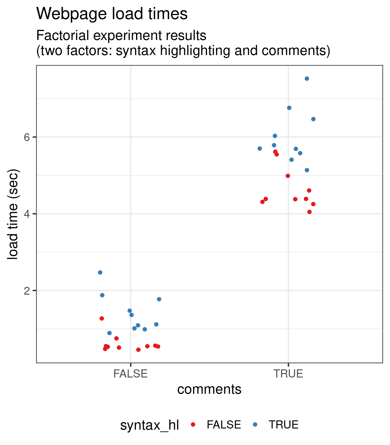
A couple of things we notice from the graph: Disqus comments and Syntax highlighting both have substantial effects on page load time. As load times increase, so does the variance in load times, which might indicate that a heteroskedastic model or log normal model is appropriate. We can also see the comments are a much greater contributor to load time than syntax highlighting.
Model Fit
Let’s test the effects of our factors. We need to fit an analysis of variance model. There are a
couple of options to do this. If we take the heteroskedasticity very seriously, we can use
oneway.test, which uses Welch’s extension of the classical (constant variance) anova, or
nlme::gls. Otherwise, we can just use lm or aov. From the plot, I do not think there is an
interaction effect between syntax highlighting and Disqus comments, but I will include it in the
model anyway (because that’s what was planned). A great thing about R is that all of these
statistical methods are included in a base installation.
Let’s try lm:
fit <- lm(loadtime ~ . * ., data = dat)
summary(fit)
##
## Call:
## lm(formula = loadtime ~ . * ., data = dat)
##
## Residuals:
## Min 1Q Median 3Q Max
## -0.8690 -0.3160 -0.1000 0.1815 1.5110
##
## Coefficients:
## Estimate Std. Error t value Pr(>|t|)
## (Intercept) 0.6200 0.1676 3.699 0.000718 ***
## commentsTRUE 4.0340 0.2370 17.019 < 2e-16 ***
## syntax_hlTRUE 0.7850 0.2370 3.312 0.002117 **
## commentsTRUE:syntax_hlTRUE 0.5700 0.3352 1.700 0.097673 .
## ---
## Signif. codes: 0 '***' 0.001 '**' 0.01 '*' 0.05 '.' 0.1 ' ' 1
##
## Residual standard error: 0.53 on 36 degrees of freedom
## Multiple R-squared: 0.9516, Adjusted R-squared: 0.9476
## F-statistic: 235.9 on 3 and 36 DF, p-value: < 2.2e-16Testing
Using the \(p\)-values, we see that comments and syntax highlighting both have an impact on load time, but the impact of comments is much greater. The interaction effect is actually not significant (I would not expect it to be).
The intercept shows me the expected load time if I disable comments and syntax highlighting, 0.62 seconds. That’s pretty fast. If I keep comments and highlighting, my load time will be 0.62+4.03+0.78+0.57= 6 seconds. That’s terrible.
The residual SD is about 0.5 seconds. That’s the average amount of noise about each mean, over all the ANOVA conditions. There are four conditions in the model. The noise is due to the network, and is actually an underestimate of the true noisiness of the website, since I only used one machine and one connection to collect the data.
The model \(R^2\) is very high, but we should not comment on that.
A better model?
Possibly of interest, we can test to see if we ought to have modeled the non-constant variance in
the data. We can use GLS to fit the model:
fit_var <- nlme::gls(loadtime ~ comments * syntax_hl, data = dat,
                     weights = nlme::varIdent(form = ~ 1 | comments * syntax_hl))
fit_var
## Generalized least squares fit by REML
## Model: loadtime ~ comments * syntax_hl
## Data: dat
## Log-restricted-likelihood: -28.28879
##
## Coefficients:
## (Intercept) commentsTRUE
## 0.620 4.034
## syntax_hlTRUE commentsTRUE:syntax_hlTRUE
## 0.785 0.570
##
## Variance function:
## Structure: Different standard deviations per stratum
## Formula: ~1 | comments * syntax_hl
## Parameter estimates:
## FALSE*FALSE TRUE*FALSE FALSE*TRUE TRUE*TRUE
## 1.000000 2.273536 2.081658 2.962239
## Degrees of freedom: 40 total; 36 residual
## Residual standard error: 0.2414309Under the new model, a different noise term is estimated for each of the experimental strata. We use
the R function anova to determine if modeling the noise terms is a much more honest representation
of the data:
fit_t <- update(fit_var, weights = NULL)
anova(fit_var, fit_t)
## Model df AIC BIC logLik Test L.Ratio p-value
## fit_var 1 8 72.57758 85.24573 -28.28879
## fit_t 2 5 75.66403 83.58163 -32.83202 1 vs 2 9.086456 0.0282The small \(p\)-value indicates that the GLS model fit_var is significantly better.
But if we are only interested in the mean load times, the difference between the models is of no concern.
Conclusions
I will disable JS code highlighting and comments on this blog. While syntax highlight has a small but noticeable impact on page performance, I find that the highlighting performed is pretty low quality compared to what I get in Emacs, so we can just turn that off with very little functionality loss.
The funniest part of this whole exercise that after disabling the big JS features, my Chrome Lighthouse score actually decreased from 69 to 66! C’mon!
Can you help me?
I don’t have much experience with web dev. If you know of anything I missed that can make this website faster while maintaining comments and syntax highlighting, I’m all ears.