
We talk a lot about Bayes on the blog, because Bayes is internally coherent. But there’s also a fair amount of coherence on the frequentist side as well. The coherence in frequentist stats generally comes from the theory of estimating equations. In this post, we will start with one of the grandparents of estimating equations, the quasi-binomial model. Quasi models are a beautiful class of models that don’t assume any likelihood (!). Rather, a relationship on the mean and variance is specified, and this gives rise to some limited statistical inference.
Math
First, take comfort in the fact that binary data cannot be overdispersed. If you’ve got some 1/0 binary data with \(E(y)=p\), then there’s no place for the variance to go. The variance must be \(p(1-p)\). Binomial data are another story. We can imagine data that result in counts that do not vary according to the Binomial model.
If the data are Binomial, \(y_{j} \sim \mathrm{Bin}(n_{j}, p)\), then the first and second central moments are
\[ \mathrm{E}(y_j) = n_j p \]
and
\[ \mathrm{var} (y_j) = n_j p (1-p) \]
Realistically, this mean/variance relationship is typically not supported by the data we see. Typically data are either under-dispersed or over-dispersed, which means that the variance (as a function of \(E(y_{j})\)) is too big or too small, and so does not match what we see in the field.
A Quasibinomial model is a possible remedy in this situation. It is a good idea to rectify the dispersion problem because poor dispersion assumptions will lead to poor inferential properties: wrong confidence intervals and \(p\)-values. The Quasibinomial model adds an extra dispersion parameter to the variance, so it has slightly different central moments.
Quasi likelihood models do not specify data generating processes on the data. Rather, just the mean and variance are specified, which is enough to determine confidence intervals for parameters.
The model is motivated by studying clustered data. We follow McCullough and Nelder on this one. But note that clustering may be not be the only good motivator for over-dispersion, it’s just one that seems to be common in practice.
Suppose there are \(m\) individuals portioned into \(k\) clusters, so that each cluster is size \(n=m/k\). In the \(j^{th}\) cluster, the number of successes \(Z_j\) is assumed to follow a Binomial distribution with parameter \(\pi_j\). \(\pi_j\) can vary from cluster to cluster. The total number of positive responses is then
\[ S = \sum_j Z_j \]
IF (big if!) we further assume that \(E(\pi_{j})=\pi\) and \(\mathrm{var}(\pi_{j})=\tau^2 \pi (1-\pi)\), it can be shown that the unconditional mean and variance of \(S\) are
\[ \mathrm{E}(S) = m \pi \]
and
\[ \begin{align} \mathrm{var}(S) &= m \pi (1 - \pi) (1 + (k - 1) \tau^2) \\ &= m \pi (1 - \pi) \sigma^2. \end{align} \]
Above, we assumed the clusters are equal size, but this isn’t strictly a requirement.
Code
Here is a little example that shows the effect of dispersion modeling on GLM results. First, make some data. The data are binomial in each group, and each group has a different parameter (though this is not in the data generation process).
In regression modeling, I’m probably not interesting in \(E(S)\) and \(\mathrm{var}(S)\). Instead, I care about \(E(\pi_{j})\) and \(\mathrm{var}(\pi_{j})\). Luckily, R basically has one-liners to calculating confidence intervals for \(E(\pi_{j})\).
library(data.table)
library(ggplot2); theme_set(theme_bw(base_size = 15))

dat <- data.table(
  s = rep(c(4, 5, 10, 18, 19), each = 4),
  n = rep(20, 20))
If we fit the Binomial model, we get a confidence interval on \(\pi\):
fit <- glm(cbind(s, n - s) ~ 1, family = binomial, data = dat)
plogis(confint(fit))
## Waiting for profiling to be done...## 2.5 % 97.5 %
## 0.5110879 0.6081467More appropriately, we can use the quasi-binomial model to get the confidence
interval for \(E(\pi_{j})\). Note that the only change is to the family argument
fit_q <- glm(cbind(s, n - s) ~ 1, family = quasibinomial, data = dat)
plogis(confint(fit_q))
## Waiting for profiling to be done...## 2.5 % 97.5 %
## 0.4178741 0.6957634The interval is much wider, but is it better? To answer this question, we look at the estimate of the dispersion parameter, \(\sigma^{2}\):
summary(fit_q)##
## Call:
## glm(formula = cbind(s, n - s) ~ 1, family = quasibinomial, data = dat)
##
## Deviance Residuals:
## Min 1Q Median 3Q Max
## -3.3006 -2.8168 -0.5386 3.3398 3.9667
##
## Coefficients:
## Estimate Std. Error t value Pr(>|t|)
## (Intercept) 0.2412 0.2935 0.822 0.422
##
## (Dispersion parameter for quasibinomial family taken to be 8.492823)
##
## Null deviance: 184.03 on 19 degrees of freedom
## Residual deviance: 184.03 on 19 degrees of freedom
## AIC: NA
##
## Number of Fisher Scoring iterations: 4If the dispersion parameter is close to \(1\), there’s not much going on beyond a regular Binomial model. The parameter is 8.492823, significantly larger than 1!
There are other solid ways to model over-dispersion. A Beta-Binomial model is a full-likelihood solution to the over-dispersion problem, and has appeared on this blog in the past. Also, there are good reasons to use quasi likelihoods even when over-dispersion is not a concern. For one, a quasi model has more relaxed assumptions than comparable likelihood models.
Proportion data
A very curious feature of R’s quasi-binomial implementation is that you can feed it proportional data without specifying a numerator and denominator. This would be a problem for binomial regression, but quasi-binomial does not complain. A visual inspection of the results shows agreement with the confidence interval we calculated from the previous QB model.
dat[, prop := s / n]
fit_prop <- glm(prop ~ 1, family = quasibinomial, data = dat)
plogis(confint(fit_prop))
## Waiting for profiling to be done...## 2.5 % 97.5 %
## 0.4178741 0.6957634How can this be? Let’s code the QB model from scratch to see what’s going on.
For each observed proportion prop we can take \(E(\mathrm{prop}_{j}) = p\) and
\(\mathrm{var}(\mathrm{prop}_{j}) = p (1-p) \tau^2\).
We construct the quasi score function, \(s(\beta, \tau^{2}) = D^t V^{-1} (\mathrm{prop} - \mu(\beta))\), where \(\mu\) is the inverse logit of \(\beta\), \(D\) is the matrix of first derivatives of \(\mu\), and \(V\) is the variance-covariance matrix. See Wakefield, p. 318 for more details on this score function. To tie things nicely back to the beginning of the post, the score function is an example of an estimating function. The corresponding estimating equation is \(s(\beta, \tau) = 0\).
score_q <- function(beta, tau2, prop){
  k <- length(prop)
  mu <-  exp(beta) / (1 + exp(beta))
  dmu <- exp(beta) / (1 + exp(beta)) ^ 2
  v <-  mu * (1 - mu) * tau2
  D <- rep(dmu, k)
  V_inv <- diag(rep(1 / v, k))
  D %*% V_inv %*% (prop - rep(mu, k))
}
And find the zero of the score using a root finding algorithm:
coef(fit_prop)## (Intercept)
## 0.2411621uniroot(score_q, c(-10, 10), prop = dat$prop, tau2 = 1)## $root
## [1] 0.241161
##
## $f.root
## [,1]
## [1,] 5.124649e-06
##
## $iter
## [1] 7
##
## $init.it
## [1] NA
##
## $estim.prec
## [1] 6.103516e-05Aha! agreement with R’s built-in glm function!
We can draw a little graph that displays the score function that is traversed by uniroot:
pdat <- data.table(x = seq(-2, 2, length.out = 200))
pdat[, score := score_q(x, 1, dat$prop), by = x]

ggplot(pdat, aes(x, score)) +
  geom_line(size = 2) +
  xlab(expression(beta)) +
  geom_hline(aes(yintercept = 0), linetype = "dotted")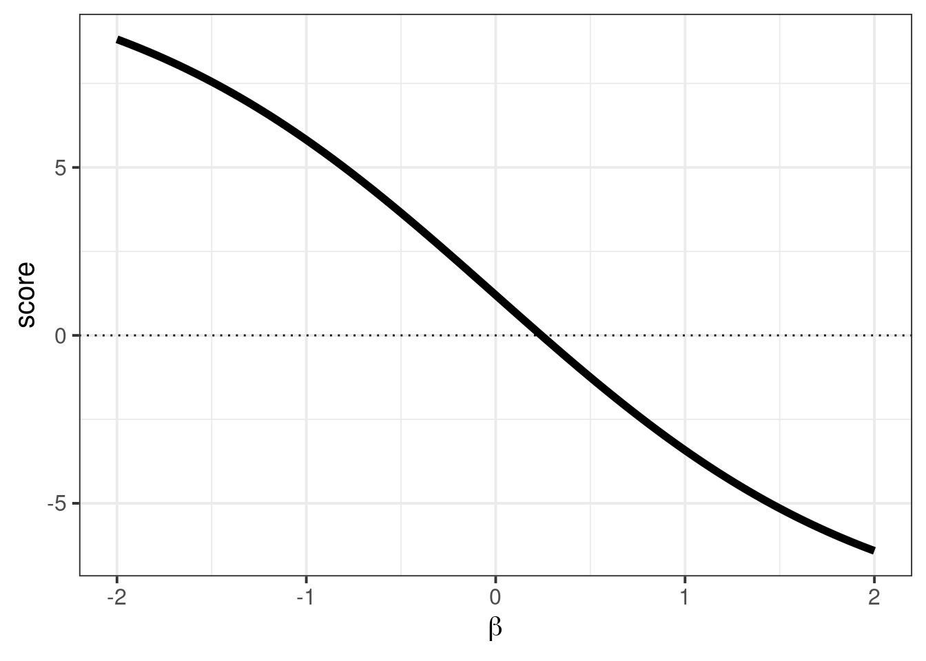
Note, that we didn’t find an estimator for \(\tau^2\). (This is outside the limitations of quasi-likelihood.) Though we can do so with a method of moments style estimator to get the variance corrected confidence intervals.
We can complete the QB calculation by calculating the dispersion parameter, \(\tau\), in this parameterization. We simply take the Pearson statistic, and divide by the degrees of freedom:
\[ \hat{\tau^2} = \frac{1}{n-1} (\mathrm{prop} - \mu)^t V^{-1} (\mathrm{prop} - \mu) \]
beta_hat <- coef(fit_prop)
n <- length(dat$prop)
mu <- plogis(beta_hat)
v <-  mu * (1 - mu)
delta <- (dat$prop - mu)
V_inv <- diag(rep(1 / v, n))

delta %*% V_inv %*% delta / (n - 1)
## [,1]
## [1,] 0.4246411The calculation reveals that the dispersion parameter is sensitive to the model parameterization, but R automatically does the right thing. It calculates \(\sigma\) when you feed the model counts and calculates \(\tau\) when you feed the model proportions.
I find it unfortunate that R’s glm function will not permit the same type of calculation with proportions when just doing plain-jane Binomial logistic regression. On the other hand, R’s stringent data requirements are good for preventing errors in the regression.
Okay, that’s all for now. Maybe next time we do confidence intervals and sandwich corrections.