
library(ggplot2); theme_set(theme_bw(base_size = 15))
library(data.table)
First, some data
dat <- data.table(
  x = gl(2, 10, 20),
  z = gl(2, 5, 20))

X <- model.matrix( ~ . * ., data = dat)

beta <- c(1, 2, 3, 1)

dat$y <- rnorm(20, X %*% beta, 1)
Plot the data:
## calculate means by each group
means <- dat[, .(m = mean(y)), by = .(x, z)]

## plot means with raw data
p <- ggplot(dat, aes(x = x, y = y, color = z, group = interaction(x, z))) +
  geom_point() +
  geom_point(data = means, aes(y = m), fill = 'black', col = "black", size = 4, shape = 21)
p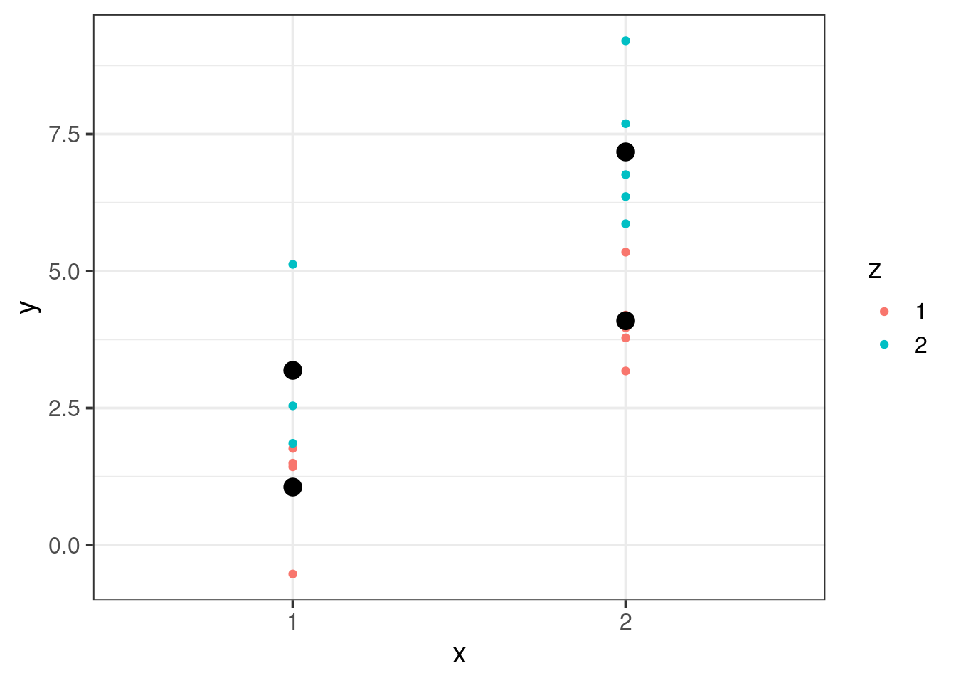
When we fit an ANOVA model, what do the coefficients mean? We can interpret them geometrically. Below, I will plot the betas visually, to show how they sum to give the group means. There is no unique way to do this, so I will just show some of the two more common versions.
The way that group means decompose to parameters in the ANOVA model is called a contrast coding.
Treatment Coding
First we set the data for plotting:
fit_treat <- lm(y ~ . * ., data = dat)
coefs <- coef(fit_treat)

smat <- unique(X)
sm <- unique(dat[, c("x", "z")])

for (j in 1 : ncol(X)) {
  set(sm, j = paste0("beta", j - 1), value = as.matrix(smat[, 1 : j]) %*% coefs[1 : j])
}

out <- melt(sm,
            id.vars = c("x", "z"),
            measure.vars = patterns("beta"),
            variable.name = "Coefficient",
            value.name = "yend")

out[, ystart := shift(yend, type = "lag"), by = .(x, z)]
out[is.na(out)] <- 0
Then render the plot:
p2 <- ggplot(means, aes(x = x)) +
  ggtitle("Treatment Coding") +
  xlab("x") +
  ylab("y") +
  geom_segment(data = out,
               aes(x = x, xend = x, y = ystart, yend = yend,
                   color = Coefficient), size = 2) +
  geom_point(aes(y = m),
             fill = 'black', col = "black", size = 4, shape = 21) +
  ylim(c(0, NA))
p2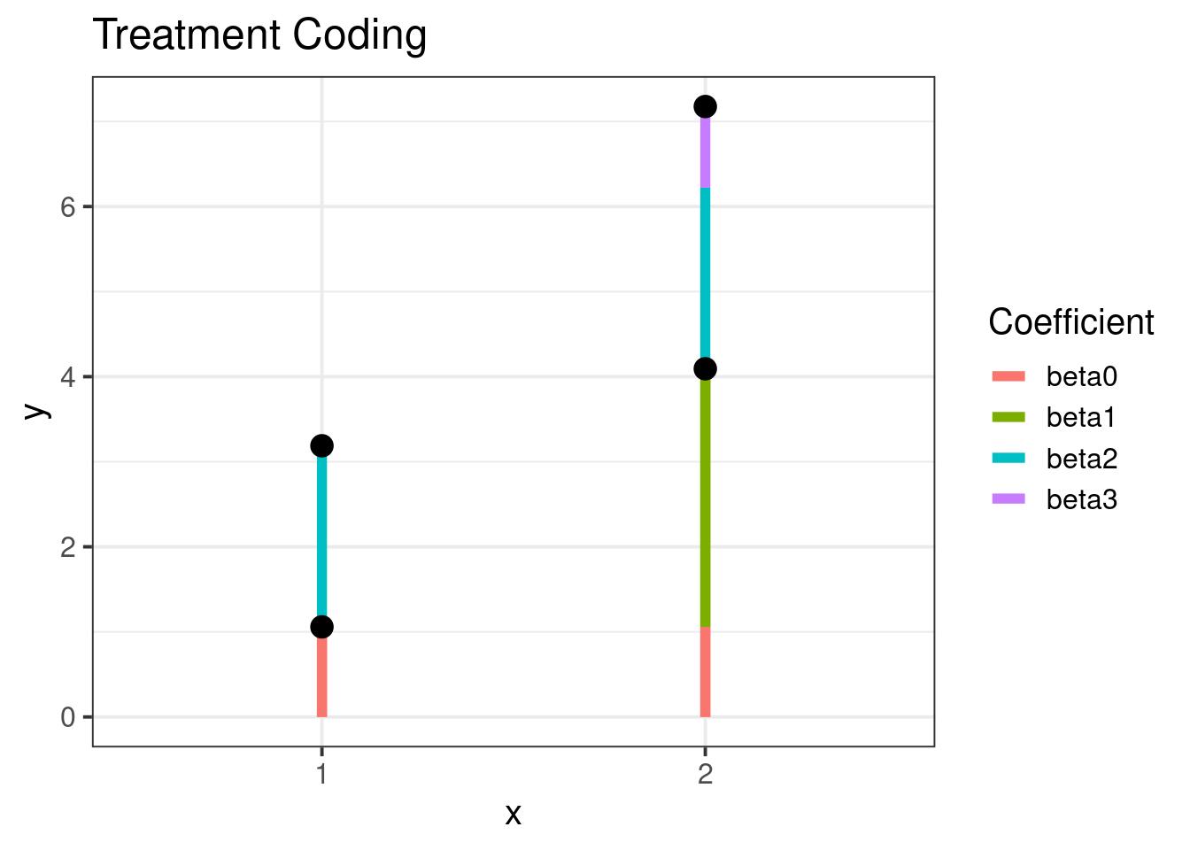
The plot shows the following treatment code relation visually:
| x level | z level | ANOVA Estimate |
|---|---|---|
| Low | Low | \(\beta_ 0\) |
| Low | High | \(\beta_0 + \beta_1\) |
| High | Low | \(\beta_0 + \beta_2\) |
| High | High | \(\beta_0\) + \(\beta_1\) + \(\beta_2\) +\(\beta_3\) |
Sum-to-Zero Coding
With Sum coding, it will look a little different.
fit_sum <- lm(y ~ . * ., data = dat,
              contrasts = list("x" = "contr.sum",
                               "z" = "contr.sum"))
coefs <- coef(fit_sum)

X2 <- model.matrix( ~ x * z, data = dat,
                   contrasts.arg = list("x" = "contr.sum",
                                        "z" = "contr.sum"))

smat <- unique(X2)
sm <- unique(dat[, c("x", "z")])

for (j in 1 : ncol(X)) {
  set(sm, j = paste0("beta", j - 1), value = as.matrix(smat[, 1 : j]) %*% coefs[1 : j])
}

out2 <- melt(sm,
             id.vars = c("x", "z"),
             measure.vars = patterns("beta"),
             variable.name = "Coefficient",
             value.name = "yend")

out2[, ystart := shift(yend, type = "lag"), by = .(x, z)]
out2[is.na(out2)] <- 0
In this case, we need to jitter the x-values to show how the coefficients sum to give the group means:
xj <- c(0, 0, 0, 0,
        -0.02, 0.02, -0.02, 0.02,
        -0.04, 0.04, -0.04, 0.04,
        -0.06, 0.06, -0.06, 0.06)
Then render the plot:
p3 <- ggplot(means, aes(x = as.numeric(x) + xj[13 : 16],
                        y = m)) +
  ggtitle("Sum-to-Zero (DOE) Coding") +
  xlab("x") +
  ylab("y") +
  geom_point(aes(y = m),
             fill = 'black',
             col = "black",
             size = 4,
             shape = 21) +
  geom_segment(data = out2,
               aes(x = as.numeric(x) + xj,
                   xend = as.numeric(x) + xj,
                   y = ystart,
                   yend = yend,
                   color = Coefficient),
               arrow = arrow(length = unit(0.2, "cm")),
               size = 2) +
  ylim(c(0, NA))
p3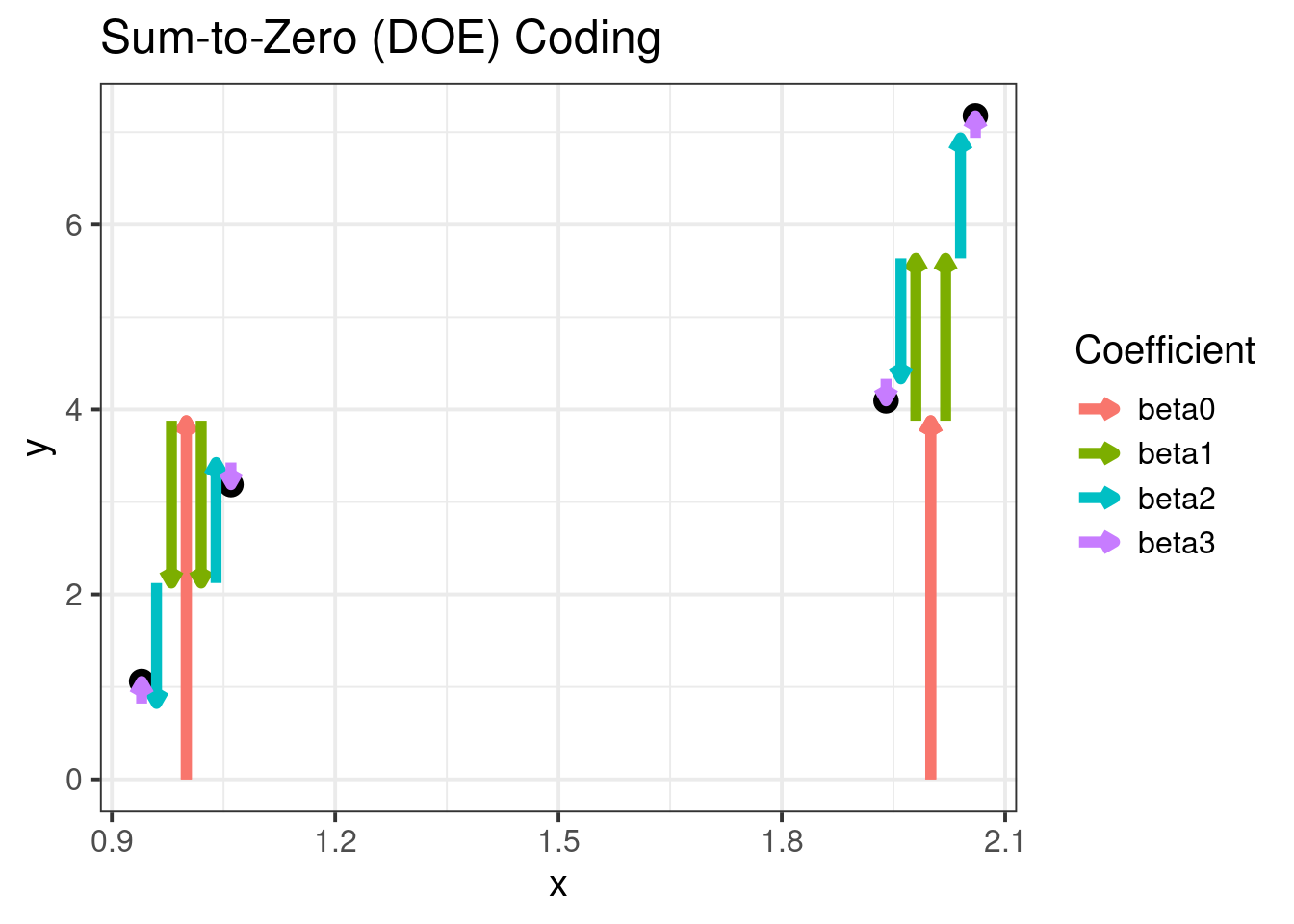
The plot shows the following DOE coding relation visually:
| x level | z level | ANOVA Estimate |
|---|---|---|
| Low | Low | \(\beta_0\) - \(\beta_1\) - \(\beta_2\) + \(\beta_3\) |
| Low | High | \(\beta_0\) - \(\beta_1\) + \(\beta_2\) - \(\beta_3\) |
| High | Low | \(\beta_0\) + \(\beta_1\) - \(\beta_2\) - \(\beta_3\) |
| High | High | \(\beta_0\) + \(\beta_1\) + \(\beta_2\) + \(\beta_3\) |