library(ggplot2); theme_set(theme_bw(base_size = 15))
library(data.table)
One thing that is statistically concerning about the current COVID situation is the multiple testing problem around vaccine trials. The New York Times is currently tracking the status of vaccines in the US and elsewhere. As of October 27, 34 are in phase 1, 13 in phase 2, and 11 are in phase 3. If we suppose that all the phase 1 and 2 vaccine candidates are safe, then there are 58 possibly effective treatments. (I will ignore the ‘limited’ and ‘approved’ vaccines for the moment.)
If there are was one vaccine candidate, there would probably not be any statistical issues, but we have 58. That’s 58 hypothesis tests that are possibly conducted in isolation. This is a huge multiplicity problem for statisticians. Multiplicity in statistics means that if we look at 58 different noisy data sources, we are likely to accidentally declare an ineffective vaccine as effective (false positive).
What’s the worst case scenario? It would be if none of the vaccines are actually effective. In that case, the probability of declaring some ineffective vaccine as effective is \(1-(0.95)^{58}\), or 0.9489531.
If none of vaccines in phase 1 or 2, make it to phase 3, then we have only 11 candidate vaccines. If none of the six phase 3 vaccines are effective, the probability of declaring some ineffective vaccine as effective is \(1 - (0.95)^{11}\), or 0.4311999.
Of course, it’s actually more likely that some proportion of the vaccines are effective (let’s have some faith after all!). In that case, it’s interesting to ask: given an effective vaccine is declared, what is the probability that we the vaccine is truly effective?
In other words, my interest is in
\[ \mathrm{Pr(Vaccine\,\,Effective | p-value < 0.05).} \]
This depends on the proportion of effective vaccines in the population of vaccines, the effectiveness of the vaccines, and how many individuals are enrolled in the trials, among possibly other variables.
Let’s start with 58 potential vaccines. Here is my simulation.
The rough idea is to generate 58 trials worth of data with a set proportion of truly effective vaccines. For each of the 58 trials, filter down the trials with \(p\)-values less than 0.05 (these are the ‘declared-effective’ vaccines). Then, on that filtered subset, determine the proportion of truly effective vaccines among the declared effective vaccines. Repeat about 500 times for each underlying proportion of truly effective vaccines.
prob_effective_given_pvalue <- function(num_trials,
                                        effectiveness,
                                        trial_size){
  prob_effective <- rep(NA, num_trials)
  dat <- data.frame(
    trial = seq_len(num_trials),
    N = trial_size,
    pvalue = NA)
  for(i in seq_len(num_trials)){
    dat$effective <- c(rep(TRUE, i), rep(FALSE, num_trials - i))
    dat$prob <- c(rep(0.5 - effectiveness, i), rep(0.5, num_trials - i))
    how_many <- rep(NA, 500)
    for(j in seq_len(500)){
      dat$S <- with(dat, rbinom(N, N, prob))
      for(k in seq_len(num_trials)) {
        dat$pvalue[k] <- with(dat, prop.test(S[k], N[k], p = 0.5))$p.value
      }
      dat_with_small_pvalue <- dat[dat$pvalue < 0.05, ]
      how_many[j] <- with(dat_with_small_pvalue,
                          if (!!nrow(dat_with_small_pvalue)) mean(effective)
                          else NA)
    }
    prob_effective[i] <- mean(how_many, na.rm = TRUE)
  }
  data.frame(prob_effective_given_pvalue = prob_effective,
             prop_effective = seq_len(num_trials) / num_trials)
}

out <- prob_effective_given_pvalue(58, 0.1, 200)
Above, I assume that there are 58 phase 3 trials, with 200 individuals enrolled in each trial. Further, I assume that an effective vaccine reduces mortality by 10%. I also (incorrectly) assume baseline mortality is 50%.
Here are the results:
ggplot(out, aes(x = prop_effective, y = prob_effective_given_pvalue)) +
  geom_point(size = 2) +
  geom_line() +
  scale_y_continuous(n.breaks = 11, limits = c(0, 1)) +
  scale_x_continuous(n.breaks = 11, limits = c(0, 1)) +
  geom_vline(aes(xintercept = 0.5)) +
  geom_hline(aes(yintercept = 0.5)) +
  xlab("Proportion of vaccines that are truly effective") +
  ylab("Probability that a declared-effective vaccine\nis truly effective") +
  ggtitle("58 trials, 10% reduction in mortality,\n200 individuals per trial")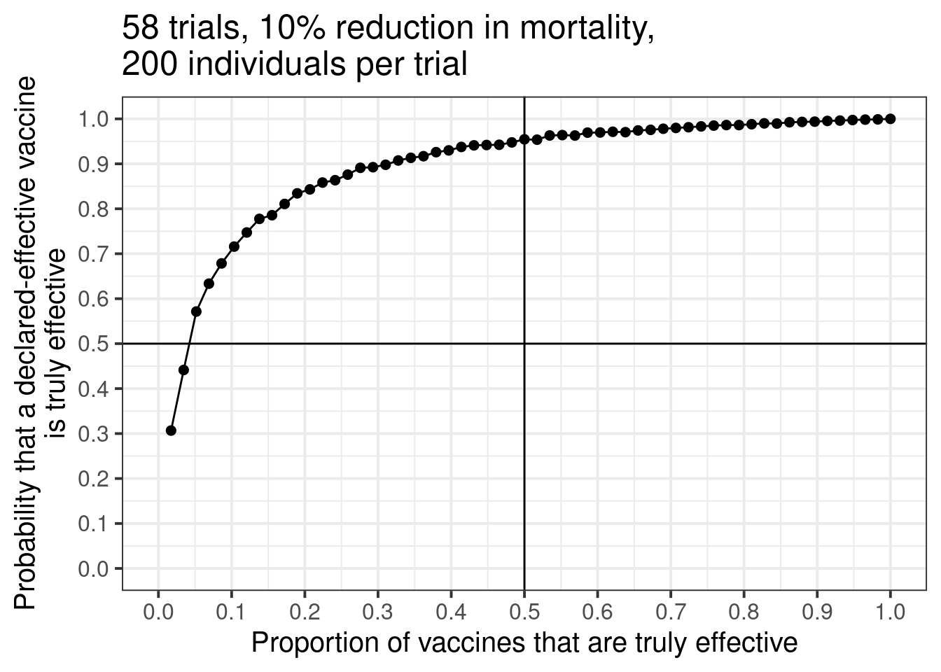
Each dot represents a simulation of 58 trials. On the left side of the graph, only one of the 58 trials is truly effective. Moving from left to right, we add one effective trial at a time until all 58 trials are effective. On the far right of the graph, because all trials are assumed truly effective, any declared effective vaccine will be truly effective.
But all the action is on the left side. There is a huge increase in vaccine confidence as the proportion of effective vaccines increase from 0 to 20%. If 20% of the vaccines are effective, the probability that a declared-effective vaccine is truly effective is about 85%. Not bad! But after this point, gains are pretty slow.
There is some noise due to simulation error, but it’s a nice picture. Unfortunately, in my simulation, if we want to be 95% confident that a declared-effective vaccine is truly effective, we need about half of the 58 vaccines to be truly effective in the first place.
An extension of this simulation would be to add a distribution on the effects of all the truly effective vaccines, as opposed to setting them to a constant.
(BTW, I’m not a biostatistician and I don’t know how many subjects will be in each trial, or the thresholds required to declare a vaccine effective. I just know a multiplicity problem when I see one!)