 is licensed under CC BY 2.0. To view a copy of this license, visit https://creativecommons.org/licenses/by/2.0/?ref=openverse&atype=rich")
Introduction
I’m interested in the model that is described in this post by Alexander Volkmann, which is a riff on a model described in Chapelle and maybe elsewhere too.
Volkmann describes a Bayesian model for an A/B test situation that uses the time to event data instead of the simple proportion of events.
Surprisingly, the Bayesian model produces an insight that is counter-intuitive, while the Frequentist analysis, a Fisher’s exact test, produces the inference that makes intuitive sense… if you take a simplistic look at the data.
The primary difference between the Frequentist model and the Bayesian model is that the Frequentist model analyzes the proportion of ad clicks within a certain time interval, while the Bayesian model analyzes the time-to-click data, and defines a successful ‘conversion’ as an observation with a finite time-to-click.
These are two different ways to look at the data, and it’s not obvious which one is ‘correct’. Which we should use depends on the primary estimand under study. But if we want compare them, we should at least do it within the same philosophy, e.g. Frequentist or Bayesian.1.
The Model
For the rest of the post, I will only focus on the intriguing censored data model that Volkmann proposes, because it may be applicable to my work as well. Let me describe the model:
The probability density function is given by
\[ Pr(x=k) = (1-p) \cdot 1_{\infty}(k) + p \cdot (\pi \cdot 1_{0} (k) + (1 - \pi) \cdot \lambda \cdot (1 - \lambda)^k \cdot 1_{\geq 0} (k)), \]
and cumulative probability density given by
\[ Pr(x \leq k) = p(1 - (1 - \pi) (1 - \lambda)^{k+1}). \]
All parameters, \(p\), \(\pi\), and \(\lambda\) must be between \(0\) and \(1\). This is the censored zero-inflated geometric model.
Here is the main idea on the model: when we make a change to a (say) website, we want to know if that change was indeed a good idea, so we run an experiment comparing the changed website with the unchanged website. The new website is worth keeping if the change generates more revenue, or ‘converts’ more users.
Rather than looking at the raw proportion of conversions in a time period, we can instead conceive of users as having a time-to-convert. Then there are two kinds of users: those that convert (in a finite amount of time) and those that convert in an infinite amount of time (which is to say they don’t convert!). Crucially, the parameter that discriminates between these two kinds of users is called \(p\) in this model, and the way things are set up, \(1-p\) proportion of users never convert, and \(p\) of them convert.
Then within the \(p\) group of users, there is a complicated model called a zero-inflated geometric model that estimates the finite conversion time. However, the parameters of the geometric model, \(\lambda\) and \(\pi\), are much less important than \(p\), because what we care about is conversions.
This is a rather exciting application of Bayesian statistics, because all the important parameters have bounded support, which means that using a flat prior2 should be agreeable to many scientists.
If the model is reasonable, then it would be quite useful for my work on detections.
If you think about a (say) radar detecting a threat, it might detect or it might not, and when it does detect we’d like to know how long it takes. So \(p\) controls the probability of detection and the other parameters of the zero-inflated geometric distribution control the distribution of detection times.
The big question is what happens when we don’t detect a threat. Is it because we never would have detected it? Or because we didn’t wait longer enough? The promise of this model is that we could parse apart these two components.
So far, so good.
Now, what’s the problem?
The problem is that we don’t get to see the people that don’t click on the ads. We only have a few days to run the experiment. Say we run the website A/B experiment for 7 days. After that 7 days is up, there are two types of users we didn’t see: those that would convert at a later date, and those that would never convert. The proportion of those two groups – neither of which we get to see – affects the estimation of \(p\).
I mentioned this much on the blog post, and on hackernews.
So, is this just another case of statistical over-engineering? Or a better way to model ad clicking (or radar detection) data?
It turns out, this is real. Even though the tail of the zero inflated distribution may be inflated, we can use the information of the length of the tail (by estimating parameters \(\lambda\) and \(\pi\)) to then estimate the parameter \(p\). It is really quite ingenious, and all the estimation happens jointly in either a Bayesian or a Frequentist model. In the examples below, I use Bayes, like Volkmann, but the original Chapelle paper uses the E-M algorithm, a Frequentist technique.
Exploration
What we can do is cook up some examples in R. Intuitively, the model is a good idea if it can recover the parameters from a known population that we control.
First, to generate data from the zero-inflated geometric distribution, I use the VGAM R package.
Originally, I attempted to use the Stan code for the inverse CDF to generate data, but this code created some negative samples, and I was unable to identify a fix, so started to look for a more reliable random number generator. I settled on VGAM, which is a package I have used in the past, and is well supported by the author.3
set.seed(1500)

library(VGAM)

## Use the rzigeom function from VGAM to create zero-inflated geometric data. Randomly change some of the obs to Inf to denote a no-conversion.

rcmod <- function(n, p, pi, lambda) {
  coin <- rbinom(n, 1, p)
  num.obs <- sum(coin > 0)
  num.cens <- n - num.obs
  obs.dat <- rzigeom(num.obs, lambda, pi)
  c(rep(Inf, num.cens), obs.dat)
}
We can use rstan to compile the model (stan code is provided on github).
I find it more convenient to define the code in two files: one file is used in the case of censoring, the other file is used in the case of no censoring.
library(rstan)I just compile the two models:
p <- "/home/john/Nextcloud/Documents/words/content/post/2022-01-12-one-strange-model/"

## one stan model w/o censoring
mod.no.cens <- rstan::stan_model(paste0(p, "my-model-no-cens.stan"))

## model w/ censoring
mod <- rstan::stan_model(paste0(p, "my-model.stan"))
Note, in Volkmann’s data, there is a variable censoring time, but in my data the censoring time is so far fixed.
Model w/o censoring
First, try to recover the geometric model parameters when there is no censoring.
dat <- rcmod(5000, 1, 0.4, 0.1)
hist(dat, breaks = 20)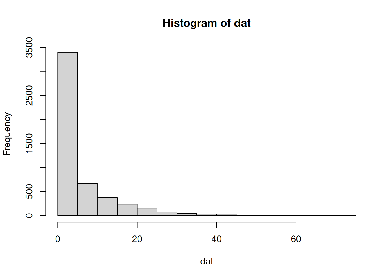
input.no.cens <- list(
  run_estimation = 1,
  N_obs = length(dat),
  N_cens = 0,
  W_obs = rep(1, length(dat)),
  W_cens = 1,
  conv_lag_obs = dat,
  elapsed_time = 0)

rstan::sampling(mod.no.cens, data = input.no.cens,
                refresh = 0)
## Inference for Stan model: my-model-no-cens.
## 4 chains, each with iter=2000; warmup=1000; thin=1;
## post-warmup draws per chain=1000, total post-warmup draws=4000.
##
## mean se_mean sd 2.5% 25% 50% 75%
## p 1.00 0.00 0.00 1.00 1.00 1.00 1.00
## pi 0.39 0.00 0.01 0.38 0.39 0.39 0.40
## lambda 0.10 0.00 0.00 0.10 0.10 0.10 0.10
## conv_lag_pred 4.54 0.16 10.00 -5.00 -2.00 1.00 8.00
## lp__ -12288.04 0.03 1.25 -12291.19 -12288.62 -12287.69 -12287.11
## 97.5% n_eff Rhat
## p 1.00 3599 1
## pi 0.41 2964 1
## lambda 0.11 3624 1
## conv_lag_pred 31.00 3967 1
## lp__ -12286.61 1549 1
##
## Samples were drawn using NUTS(diag_e) at Sat Jan 22 18:53:59 2022.
## For each parameter, n_eff is a crude measure of effective sample size,
## and Rhat is the potential scale reduction factor on split chains (at
## convergence, Rhat=1).Okay, this seems to work fine. Now we introduce censoring:
Model w/ censoring
Short censoring time
Let us first assume that 20% of customers do not convert, and that a censoring cut off is at 10 days. If the model is estimable, then we should be able to use Stan to recover the parameters \(p=0.80\).
Let’s just take a look at the data before we sample from the model.
## assume 1/5 of all customers do not convert
dat <- rcmod(5000, .8, 0.4, 0.1)

## assume a censoring time of ten days
dat.cens <- ifelse(dat >= 10, 10, dat)
hist(dat.cens, breaks = 20)
input.cens.1 <- list(
  run_estimation = 1,
  N_obs = sum(dat.cens < 10),
  N_cens = sum(dat.cens >= 10),
  W_obs = rep(1, sum(dat.cens < 10)),
  W_cens = rep(1, sum(dat.cens >= 10)),
  conv_lag_obs = dat.cens[which(dat.cens < 10)],
  elapsed_time = dat.cens[which(dat.cens >= 10)])

## should be about 80%
rstan::sampling(mod, data = input.cens.1,
                refresh = 0)
## Inference for Stan model: my-model.
## 4 chains, each with iter=2000; warmup=1000; thin=1;
## post-warmup draws per chain=1000, total post-warmup draws=4000.
##
## mean se_mean sd 2.5% 25% 50% 75%
## p 0.72 0.00 0.01 0.70 0.71 0.72 0.73
## pi 0.44 0.00 0.01 0.42 0.43 0.44 0.45
## lambda 0.13 0.00 0.01 0.11 0.13 0.13 0.14
## conv_lag_pred 1.43 0.10 5.93 -4.00 -2.00 -1.00 3.00
## lp__ -8402.70 0.03 1.20 -8405.83 -8403.27 -8402.39 -8401.81
## 97.5% n_eff Rhat
## p 0.75 1538 1
## pi 0.46 1736 1
## lambda 0.15 1638 1
## conv_lag_pred 19.00 3734 1
## lp__ -8401.30 1747 1
##
## Samples were drawn using NUTS(diag_e) at Sat Jan 22 18:55:10 2022.
## For each parameter, n_eff is a crude measure of effective sample size,
## and Rhat is the potential scale reduction factor on split chains (at
## convergence, Rhat=1).And there it is, the model was able to correctly recover the population parameters in this case. Due to random sampling, we can get estimates with large standard errors or considerable bias, but if taken as an indicator or a component of evidence, I see the utility of the model!
Just to demonstrate that we do need to use the zero-inflated geometric data, here is the actual proportion of censored obs. It is far from 20%.
## Prop. of censored data
input.cens.1[["N_cens"]] / 5000
## [1] 0.365Appendix
I use a slightly modified Stan file from Volkmann. Here is the code from the censored data version, which is the most complicated experiment that I ran:
functions{
  real uncensored_lpmf(int y, real pi, real p, real lambda){
    if (y == 0)
      return log(p) + log(pi + (1 - pi) * lambda);
    else
      return log(p) + log(1 - pi) + log(lambda) + y * log(1 - lambda);
  }

  real censoredccdf(real y, real pi, real p, real lambda){
    return log(1 - p + p * (1 - pi) * pow(1 - lambda, y + 1));
  }

  real invcdf(real u, real pi, real p, real lambda){
    if (u > p)
      return -1;
    else
      return ceil(log( (p - u) / (p * (1 - pi)) ) / log(1 - lambda) - 1);
  }

  real uncensored_rng(real pi, real p, real lambda) {
    real u;
    u = uniform_rng(0, 1);
    return invcdf(u, pi, p, lambda);
  }
}

data {
  int<lower=0, upper=1> run_estimation;
  int<lower=0> N_obs;
  int<lower=0> N_cens;
  int<lower=0> W_obs[N_obs];
  int<lower=0> W_cens[N_cens];
  int<lower=0> conv_lag_obs[N_obs];
  int<lower=0> elapsed_time[N_cens];
}

transformed data {
  int<lower = 0> N = N_obs + N_cens;
}

parameters {
  real<lower=0, upper=1> p;
  real<lower=0, upper=1> pi;
  real<lower=0, upper=1> lambda;
}

model {
  p ~ uniform(0, 1);
  pi ~ uniform(0, 1);
  lambda ~ uniform(0, 1);

  if (run_estimation == 1) {
    for (i in 1:N_obs) {
      target += W_obs[i] * uncensored_lpmf(conv_lag_obs[i] | pi, p, lambda);
    }
    for (i in 1:N_cens) {
      target += W_cens[i] * censoredccdf(elapsed_time[i], pi, p, lambda);
    }
  }
}

generated quantities {
  real conv_lag_pred = uncensored_rng(pi, p, lambda);
}