Sampling from the Wilson score confidence distribution

library(binom)
library(HDInterval)

If you’ve worked with Binomial data for a project, you might know that there’s about 10 different ways to calculate a confidence interval for the Binomial proportion. The Wilson score interval is one of those methods. It’s appealing for a lot of problems because it’s asymmetric, does not extend outside of [0,1], and it doesn’t yield zero-width intervals.

It’s also generally applicable when the data look quasi-binomial. For instance, if you have 4.1 successes out of 5 trials, I sometimes call that quasi-binomial data. This probably sounds very strange, but there’s some situations where maybe we observe 41 successes during 50 trials, but the “information value” of the 50 trials is judged to be more like 5 independent trials.

So, there’s a few reasons to use the Wilson score interval. Usually, I’m an Agresti-Coull kind of guy, but the Wilson interval is quite common.

I was curious how I might draw samples from the distribution that corresponds to the confidence bounds of the Wilson score confidence intervals. The idea is to determine the distribution for which the quantiles match the ends of the confidence intervals. So, the 50th percentile matches the 0th- level confidence interval, the 45 and 55th percentiles match the ends of the 10th-level confidence interval, … and so on. It’s a distribution determined by the confidence interval method completely. This is not a posterior distribution, or a distribution for the binomial proportion, but I was interested in characterizing it anyway.

It turns out to be rather easy in R. The steps are

1. Collect the set of (say) 1000 confidence bounds.
2. Determine the empirical cumulative density function of the bounds.
3. Invert that, and use the inverse probability sampler to get data.

Here is an example:

confidence_levels <- seq(0, 1, 0.001)
lower <- upper <- rep(NA, 1000)
x <- 4.1
n <- 5

# 1. Collect confidence bounds
for (i in 1:1000) {
  out <- binom.confint(x, n, confidence_levels[i], "wilson")
  lower[i] <- out$lower
  upper[i] <- out$upper
}

quantiles <- c(rev(lower), upper)

# Roughly sketch the "confidence distribution"
plot(density(quantiles))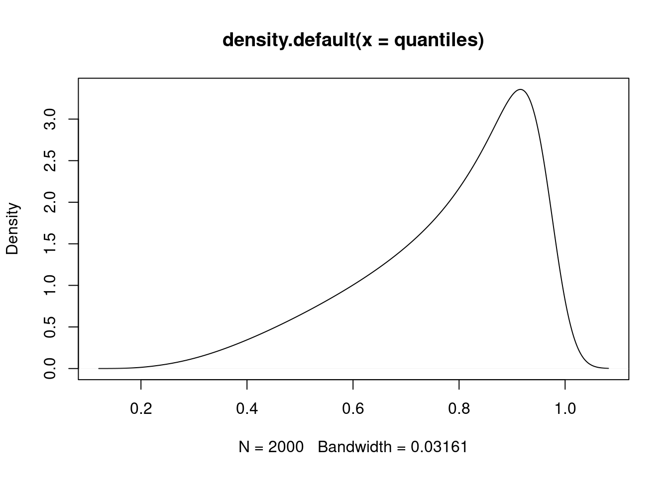

# 2. Calculate ECDF of confidence bounds
s <- ecdf(quantiles)
u <- runif(10000)

# 3. Get the samples
samps <- inverseCDF(u, s)

# We can inspect
hist(samps, breaks = 100, xlim = c(0, 1))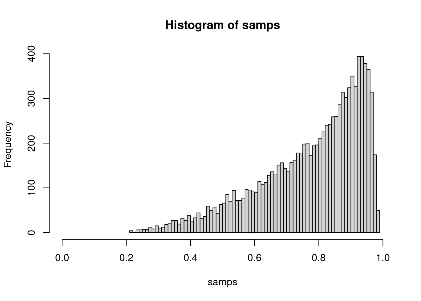

All in all, not too bad. So, if you want to characterize and sample from the “Wilson distribution” for 4.1 out of 5 successes, this is one way to do it.