Ranking is a statistical application that sorts clustered data. The goal is to find the best ordering of the groups. A common application of ranking involves Amazon resellers: When given the choice to purchase an identical product from one of several resellers, which one is the most credible? Which is the second most credible? And so on..
A naive, but noisy, way to rank resellers would simply be to rank them in order according to their average reviews. But this can get upended when a new resellers joins the marketplace and acrues a single 5 star review, putting her at the top of the list. There is a tension between the number of reviews a reseller receives and the average score of the those reviews that needs to be balanced to produce a good ranking of resellers.
Ranking is not a new statistical practice. It goes way back to the 50s, maybe futher. One of the early applications of ranking comes from estimation of genetic merit of quality of a unit. See this paper from GK Robinson on the applications of random effects to this issue, and many others.
I want to write this post to detail three methods of statistical ranking that come to mind.
Ranking by the lower bound of a confidence interval. For example, this post from Evan Miller.
Ranking by the random effect of a full model
Ranking Bayesianly, possibly using an empirical bayes approach.
The three methods are stated a bit vaguely, but can be applied whether your data is binomial, continuous, or ordinal. In this post, I’ll stick to binomial data for my simulation, but ordinal data is not so different, but common, since so many things on the internet are a 5 star rating scale.
Method 1: Lower bound of a confidence interval
This is pretty straightforward. We take the estimate of the proportion of successes in each group and compute a confidence interval. This method does not shrare information between the groups of data, for better or worse. There’s about 10 or 20 ways to compute a confidence interval for a binomial proportion, so I won’t get into that in this post, and just take the Agresti-Coull interval as the confidence interval.
library(ggplot2)
library(magrittr)
library(dplyr)
##
## Attaching package: 'dplyr'## The following objects are masked from 'package:stats':
##
## filter, lag## The following objects are masked from 'package:base':
##
## intersect, setdiff, setequal, unionset.seed(4850)
theme_set(theme_bw(base_size = 18))
nsamp <- 300
group_id <- sample(10, nsamp, replace = TRUE)
probs <- pnorm(scale(group_id))
outcome <- rbinom(nsamp, 1, prob = probs)
pdat <- data.frame(group_id = unique(group_id),
prob = unique(probs))
dat <- data.frame(group_id = group_id,
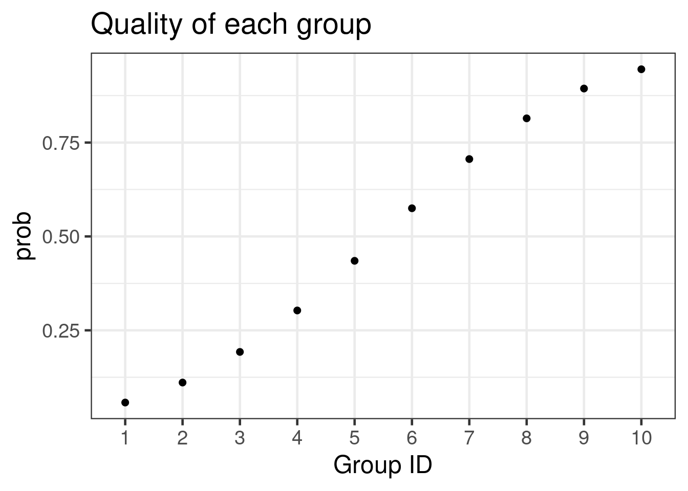
outcome = outcome) %>% arrange(group_id)The above data generation assumes groups are approximately equally sized, but in general this assumption should be relaxed. The group probabilities are graphed:
ggplot(pdat, aes(x = as.factor(group_id), y = prob)) +
  geom_point(size = 2) +
  xlab("Group ID") +
  ggtitle("Quality of each group")
Obviously the true ranking of the groups is 10, 9, 8,…
We calculate the Agresti-Coull CI for each group
library(binom)

est <- dat %>% group_by(group_id) %>%
  summarize(lower = binom.confint(sum(outcome), n(), method = 'ac')$lower,
            m = mean(outcome)) %>% arrange(lower)

est
## # A tibble: 10 x 3
## group_id lower m
## <int> <dbl> <dbl>
## 1 1 0.0278 0.103
## 2 2 0.0318 0.115
## 3 3 0.0561 0.139
## 4 4 0.159 0.290
## 5 5 0.265 0.429
## 6 6 0.345 0.5
## 7 7 0.520 0.7
## 8 8 0.520 0.7
## 9 9 0.746 0.95
## 10 10 0.799 0.941Unfortunately some lower bounds are negative, but that does not matter for ranking. The Agresti-Coull method was able to get most of the ranking correct. Good!
Ranking by random effects
Alternatively, we can fit a mixed effects model, and use the values of the estimated random effects to determine the ranking. This is a bit difficult in practice, because we may find that the mixed effects model fails to converge (a very common problem, based on personal experience and the number of questions about it on Cross Validated).
Since we have binomial data, it makes sense to fit a Bernoulli model with a single random effect for group. This can be done with lme4:
library(lme4)## Loading required package: Matrixfit <- glmer(outcome ~ (1 | as.factor(group_id)), data = dat,
family = "binomial")## boundary (singular) fit: see ?isSingularThe estimated group effects can be extracted from the fit and sorted:
re <- data.frame(group_id = unique(group_id),
                 est = ranef(fit)) %>% arrange(est.condval) %>%
  select(group_id, est.condval)

re
## group_id est.condval
## 1 2 -2.823333e-14
## 2 9 -2.393333e-14
## 3 6 -1.346667e-14
## 4 3 -1.300000e-14
## 5 8 -1.160000e-14
## 6 1 -5.333333e-15
## 7 10 -1.600000e-15
## 8 5 2.223333e-14
## 9 7 3.700000e-14
## 10 4 3.793333e-14The ordering is quite bad considering the data is fairly benign. I would have expected a ranking similar to that of the confidence interval method, but it makes little sense that group 9 is so low.
Bayesian ranking with the beta distribution
Finally we might fit a bayesian model that fits a beta distribution to each of the groups. We could use an empirical bayes (EB) or hierarchical bayes (HB) method of shrinking. For sake of demonstration, we’ll take the EB approach.
The basic idea of EB, has been best expressed by Brad Efron: If you have enough data, it naturally contains its own prior information. Here, Dr. Efron is speaking from a strictly non-subjective Bayes POV, where he considers the prior to be the best place to shrink unstable estimates towards.
In our example, we will form a Beta distribution prior by pool all the probs across all groups together, and finding the best distribution that fits those probs. With that distribution in hand, we use it as the prior for the (independent) Binomial likelihoods of each group, and update each group estimate Bayesianly.
The group probs are:
gp <- dat %>% group_by(group_id) %>% summarize(m = mean(outcome)) %>% pull(m)The Beta distribution that best fits this collection of probabilities is:
library(MASS)##
## Attaching package: 'MASS'## The following object is masked from 'package:dplyr':
##
## selectbf <- fitdistr(gp, densfun = "beta", start = list(shape1 = 1, shape2 = 1))
bf$estimate## shape1 shape2
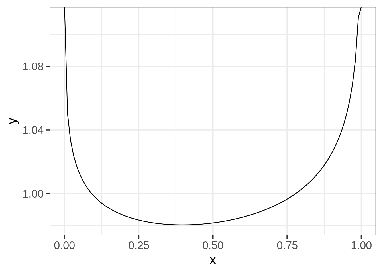
## 0.9764367 0.9642682The fitted beta distribution is extremely odd: both parameter estimates are close to 1, we can make a graph of the EB prior:
ggplot(data.frame(x = c(0, 1)), aes(x = x)) +
  stat_function(fun = "dbeta", args = list(shape1 = bf$estimate[1], shape2 = bf$estimate[2]))
Measuring disagreement from the true ranking
We need to pick a statistic that measures the discrepancy between the estimated ranking and the true ranking. This let’s us compare the three methods. I’m not an expert on rankings, but it seems like a good application for Kendall’s \(\tau\), a non-parametric measure of montonicity. Spearman’s \(\rho\) might be a good measure as well.
Simulation
Okay, I’m out of steam. But the next step is to write a small simulation.