This post is a short R demonstration on how to make fake data from three statistical models. All models are different in that each model is usually taught or encountered in a different context. But they are all the same because each model involves the generation of a “latent” normal random variable.
I am struck by the ubiquity of the latent random normal variable. It is useful for
- Time series data (Model 1)
- Distance correlated data (Model 2)
- clustered data (Model 3)
library(MASS)
library(ggplot2)
theme_set(theme_bw(base_size = 16))
Model 1
Random draw from a multi-normal with a time-series like correlation matrix:
n <- 100
x <- seq(0, 1, length = n)
Sigma <- .7 ^ as.matrix(dist(x))
y <- mvrnorm(1, mu = rep(0,n), Sigma = Sigma)
dat1 <- data.frame(x, y)
ggplot(dat1, aes(x, y)) +
geom_line() +
ggtitle("Example Time Series")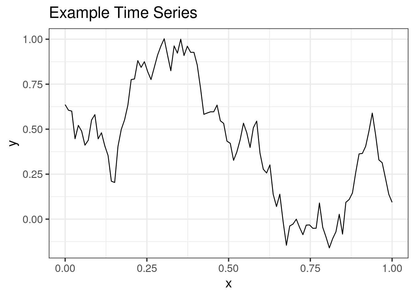
Model 2
Random draw from a multi-normal with the ‘usual’ correlation matrix:
x <- seq(0, 10, length = n)
d <- as.matrix(dist(x)) ^ 2
Sigma <- exp(-d)
y <- mvrnorm(1, mu = rep(0, n), Sigma=Sigma)
dat2 <- data.frame(x = x, y = y)
ggplot(dat2, aes(x, y)) +
geom_line() +
ggtitle("Example Gaussian Process")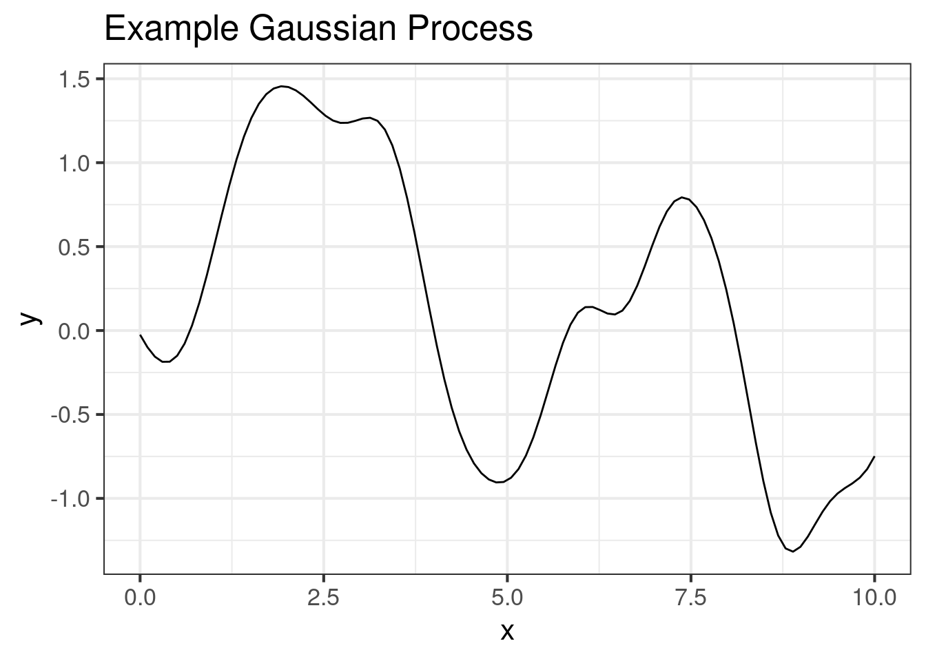
Model 3
Random draw from a multi-normal matrix (no correlations)
b0 <- 1
var_b <- 1
n_re <- 10

D_re <- model.matrix( ~ gl(n_re, n / n_re) - 1)

b <- mvrnorm(1, rep(0, n_re),
             Sigma = var_b * diag(rep(1, n_re)))

y <- b0 + D_re %*% b + rnorm(n)
dat3 <- data.frame(Factor = gl(n_re, n / n_re), y = y)
ggplot(dat3, aes(x = Factor, y)) +
geom_point(position = position_jitter(width = 0.1)) +
ggtitle("Example Random Effect Data")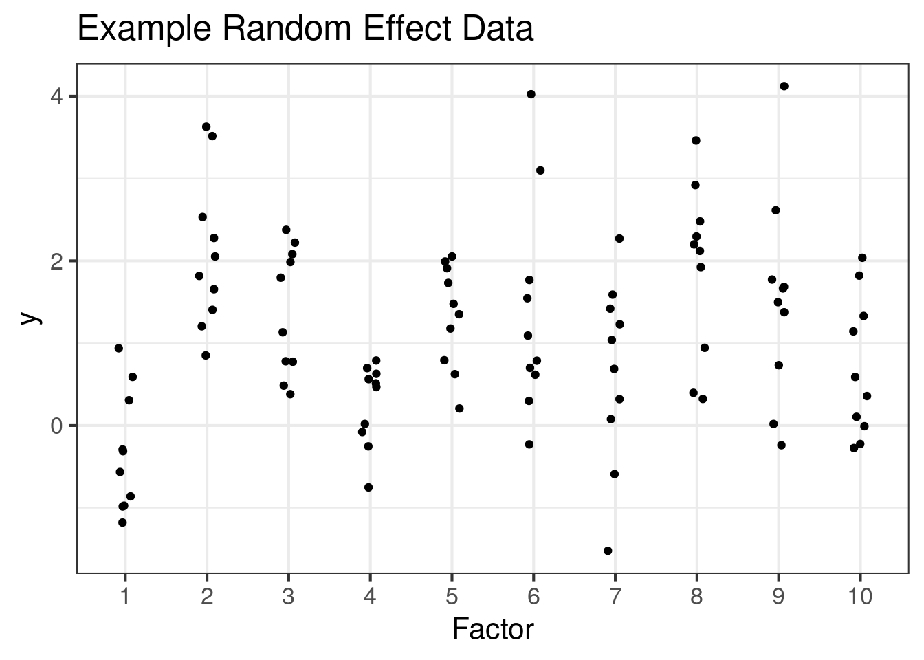
In a sense, I might just call all of these models “random effects” models, because the glmmTMB package can estimate parameters for all of these situations.