Visualizing the log determinant surface

A small simulation that shows how the volume of the linear model covariance matrix can change under sample size and factor correlations:

library(MASS)
library(data.table)

save_det <- data.table(sample_size = rep(1 : 100 + 5, each = 100),
                       corr = rep(0 : 99 / 100, 100),
                       det = NA)

det1 <- vector("numeric")

for (i in 1 : 100 + 5) {
  for (j in 0 : 99) {

    S <- matrix(c(1, j / 100, j / 100, 1), nrow = 2)
    X <- mvrnorm(i, c(0, 0), S)
    beta <- c(1, 2, 3)
    y <- cbind(1, X) %*% beta + rnorm(i)

    fit <- lm(y ~ X)

    det1 <- c(det1, det(vcov(fit)))
  }
}

save_det[, det := det1]

with(save_det,
     filled.contour(z = xtabs(log(det) ~ sample_size + corr),
                    x = unique(sample_size),
                    y = unique(corr),
                    xlab = "Sample Size",
                    ylab = "Correlation between factors",
                    color.palette = function(n) hcl.colors(n, "Spectral", rev = TRUE),
                    main = "Magnitude of log(determinant)"))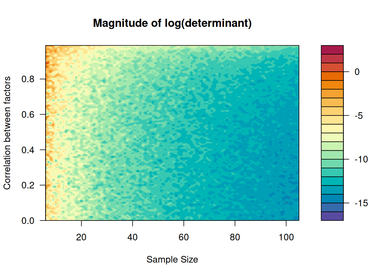

Clearly, inference is more precise under large sample sizes and small correlations.