Does model selection bias p-values?

YES.

Model selections techniques have the potential to wreck inferential statistics.

My friend brought up an interesting practice at her work: Model builders were using step-wise AIC to select a linear model specification. There are dozens of possible variables, and there is little interest in trying to select a reasonable model based on subject matter expertise. After the best model is found using step-wise selection, \(p\)-values are further called in to pare down the model: predictors with large \(p\)-values get tossed out.

I quipped that this is kinda contradictory to step-wise selection with AIC since

1. It’s possible that further refinements to the model after the step-wise selection can actually increase of the AIC.

2. Step-wise model selection invalidates the \(p\)-values reported after the fact.

The second quip is something that doesn’t get reported enough in the stats literature, and it’s not unique to step-wise methods. Any sort of data-driven model selection is going to mess up the \(p\)-values (and the confidence intervals, and the prediction intervals, and probably some other stuff too.)

In a nutshell, by optimizing for AIC, we are minimizing the \(p\)-values, because among some classes of models, small AIC is “correlated”¹ with a small set of small \(p\)-values.

I don’t mean to pick on step-wise regression in this note, it’s just one example of how modern data-mining techniques generally ruin the replicability of results. Inference after data-mining is double dipping the data: We first use the data to calculate the model that best fits the data, then we ask the model if it has found anything note worthy. But when we ask the model if it found anything good, we can forget that we already gave it the best chance to find something through data dredging!

When we do the second step (inference), virtually all statistical software forgets that we had the first (model selection) and happily reports back the \(p\)-values assuming that the final model was the first model we tested!²

Here is a small simulation to demonstrate the problem:

## Load libs
library(MASS)
library(ggplot2); theme_set(theme_bw(base_size = 15))

To start, we use 6 uncorrelated and continuous covariates.

## Specify the true model
P <- 6
beta <- seq(0, 0, length.out = P)
N <- 100

X <- mvrnorm(n = N, mu = rep(0, P),
             Sigma = matrix(0.0, P, P) + diag(1.0, P))

## do a fake model fit to pull out some useful information
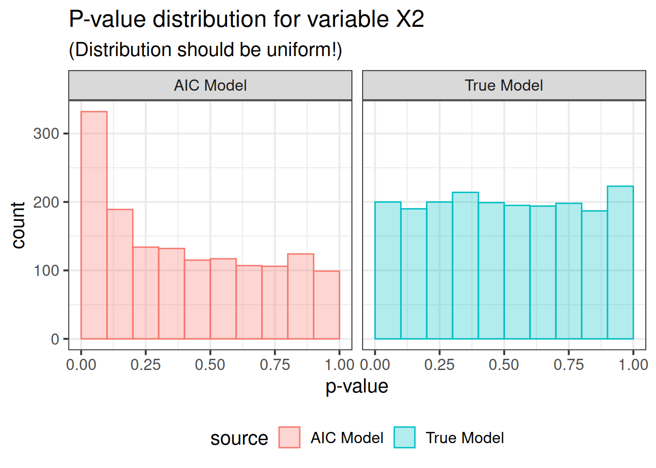
test_fit <- lm(rnorm(N) ~ X)

Now for the simulation. The basic idea is commented in the code. We’re going to keep the design matrix \(X\) constant, but in each of the \(2000\) replications, we generate a new \(y\). The true model is that none of the predictors have any effect on the outcome. That part is critical – no effect means the \(p\)-values from the true model should be uniform. At the end of the simulation, we tabulate the \(p\)-values for all the predictors into one data.frame, appending the source of the \(p\)-values, whether from a true model or from an AIC-selected model.

Now, I’m taking the easy way out by making the predictors meaningless in the true model. That’s just because I happen to know that the \(p\)-value distribution should be uniform in that case. We could cook similar examples where the true effect do matter, but I’m not sure how to work out the \(p\)-value distribution in that case.³. Either way, predictors effective or not, the model selection is going to pull the \(p\)-values closer to zero.

nsim <- 2000

## for each i
#### generate new y (X stays same, beta stays same, N same),
#### step wise regression to find best model
#### look at the p-value distr. of MEs 2, 4, and 6

out <- correct <- data.frame(matrix(vector(), nsim, P + 1))
colnames(out) <- colnames(correct) <- names(coef(test_fit))

## small helper function to pull out the p-values
get_pvals <- function(fit) summary(fit)[["coefficients"]][, 4]

for (i in 1 : nsim) {
  ## Make Data
  y <- rnorm(N, X %*% beta + 1, 1)
  DF <- data.frame(X = X, y = y)
  ## Record correct P-values
  fit <- lm(y ~ . , DF)
  correct[i, ] <- get_pvals(fit)
  ## Record AIC T-values
  fitAIC <- stepAIC(lm(y ~ . * ., DF), direction = "backward", trace = 0)
  coef_aic <- rep(1, P + 1); names(coef_aic) <- names(coef(fit))
  coef_aic <- get_pvals(fitAIC)[names(coef(fit))]
  out[i, ] <- coef_aic
}

## merge the simulation data for graphing

out$source <- "AIC Model"
correct$source <- "True Model"

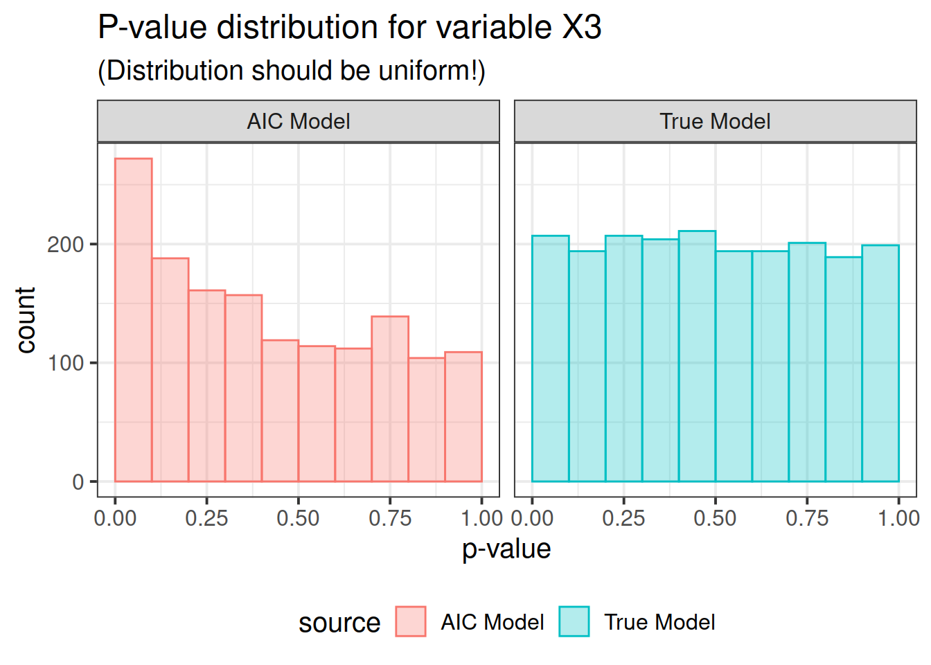
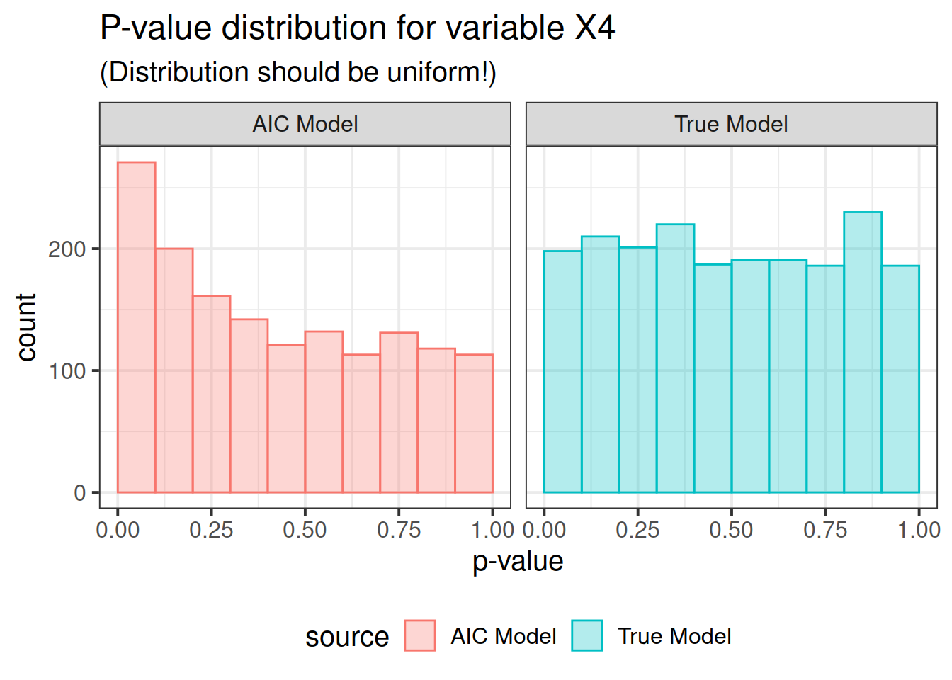
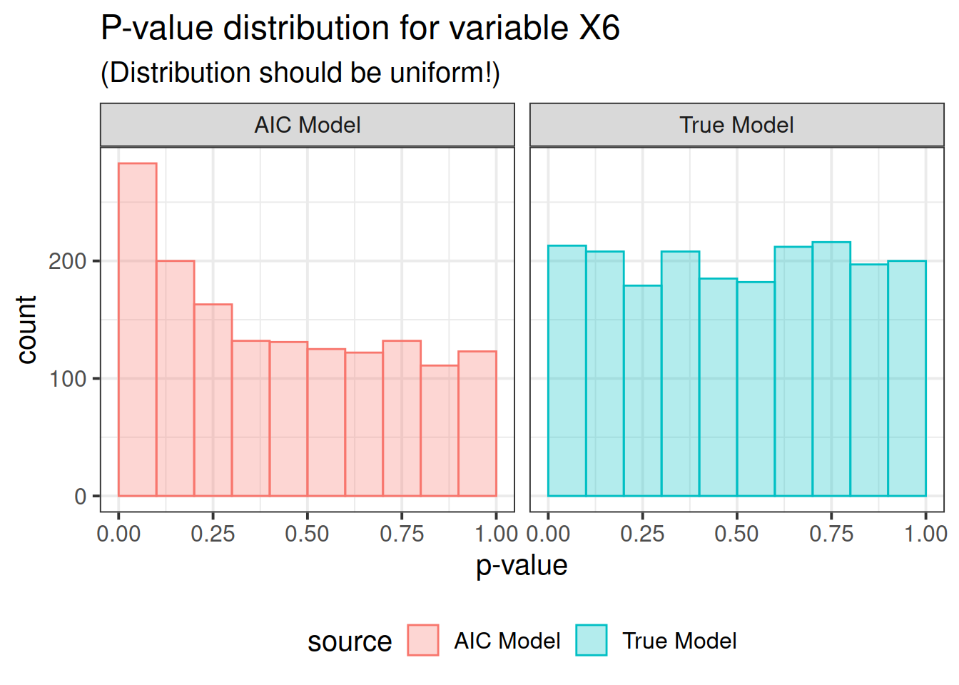
pdat <- rbind(correct, out)

Now here is the real outcome: we graph the \(p\)-value distributions for all the main effects.

We see that the data-driven step-wise selection is able to pick up some signal where none is present: the \(p\)-value distributions after step-wise selection are not flat, they are biased toward 0. This means that \(p\)-values after model selection can appear smaller than they actually are.

ppval <- function(x) {
  ggplot(pdat, aes(x = get(x), color = source, fill = source)) +
    geom_histogram(alpha = 0.3, position = "identity", breaks = seq(0, 1, 0.1)) +
    xlab("p-value") +
    ggtitle(paste("P-value distribution for variable", x),
            "(Distribution should be uniform!)") +
    facet_grid( ~ source) +
    theme(legend.position = "bottom")
}

for (i in paste0("X", 1 : P)) {
  print(ppval(i))
}

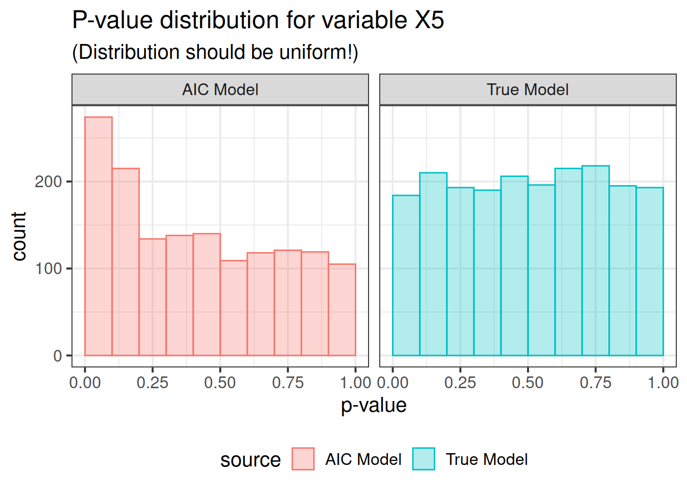
So there you have it folks. If you use data driven model selection strategies, don’t take those \(p\)-values too seriously!