
library(mvtnorm)
library(brglm2)
library(data.table)
library(ggplot2); theme_set(theme_bw(base_size = 14))
Introduction
Firth’s adjustment is a technique in logistic regression that ensures the maximum likelihood estimates always exist.
It’s an unfortunate fact that MLEs for logistic regression frequently don’t exist. This is due to sparsity in the data, which makes certain classes perfectly separable. Perfect separation is bad news for logistic regression, because it means the change in log-odds from one category to the next is infinite. The solution is Firth’s adjustment, which applies a couple corrections to either the likelihood function or the score function to ensure that MLEs are always finite.
Sounds great!1
In trying to understand Firth’s correction a bit better, I found this very illuminating stack exchange answer:
Firth’s correction is equivalent to specifying Jeffrey’s prior and seeking the mode of the posterior distribution. Roughly, it adds half of an observation to the data set assuming that the true values of the regression parameters are equal to zero.
Lots of things come to mind here:
I didn’t know Jeffrey’s prior was applicable to regression models. A bit of googling reveals that in most regression models, it is not. The Jeffrey’s prior is usually not proper. Binomial regression is a special case where it is.
This is an interesting case of a prior that depends on a model matrix. That is, \(\pi(\boldsymbol{\beta}|X) \neq \pi(\boldsymbol{\beta})\).
Can we verify this?
Jeffrey’s prior is determined by the form of the likelihood. It’s the square root of the determinant of the Fisher information matrix. In mathy words,
\[ \pi (\boldsymbol{\beta} | X) \propto \{ \mathrm{det}(X ^ \intercal W_{\boldsymbol{\beta}} X) \} ^ {1/2}. \]
where \(X\) is the design matrix, and \(X ^{\intercal} W X\) is the Fisher information matrix of the logistic regression model.
The goal of this post is to figure out how to sample from the posterior
distribution of this logistic model, and compare it to the state-of-the-art
Firth estimates given by brglm or brglm2.2
Most of the math equations in this post I found in this article.
The likelihood for logistic regression is given by
\[ L(\boldsymbol{\beta}|X,y) = \prod_{i=1}^N {n_i \choose y_i} \{ F(\boldsymbol{x}_i ^ \intercal \boldsymbol{\beta})\} ^ {y_i} \{ 1 - F(\boldsymbol{x}_i ^ \intercal \boldsymbol{\beta})\} ^ {n_i - y_i}, \]
where
\(\boldsymbol{\beta}\) is the vector of regression coefficients,
\(y = y_1, \ldots, y_N\) is the vector of binomial responses,
\(X ^{\intercal} = [\boldsymbol{x}_{1}, \ldots, \boldsymbol{x}_{N}]\) is the design matrix,
\(N\) is the total number of observations,
\(F\) is the CDF of the logistic distribution, and
\(n_i\) is in the size of each bucket.3
The \(n_i \choose y_i\) term can safely be ignored in most statistical applications, because it is not a function of \(\boldsymbol{\beta}\).
The matrix \(W\) has a nice form as well. It is diagonal, and each element is given by
\[ w_i(\boldsymbol \beta) = \frac {n_i \{ f (\boldsymbol{x} ^ \intercal _ i \boldsymbol{\beta})\} ^ 2} { F(\boldsymbol{x}_i ^ \intercal \boldsymbol{\beta}) \{ 1 - F(\boldsymbol{x}_i ^ \intercal \boldsymbol{\beta})\} }, \]
where \(f\) is the PDF of the logistic distribution. It might be more stable to compute this matrix on the log-scale, but in my examples, this made no difference. The log-scale \(W\) matrix has diagonal entries
\[ \log(w_i(\boldsymbol{\beta})) \propto 2 \log(f (\boldsymbol{x} ^ \intercal _ i \boldsymbol{\beta})) - \log(F (\boldsymbol{x} ^ \intercal _ i \boldsymbol{\beta})) - \log (1 - F(\boldsymbol{x} ^ \intercal _ i \boldsymbol{\beta})). \]
(I omitted the \(n_i\) term because it doesn’t make a difference for Bernoulli logistic regression.)
Visualizing the Prior
Let’s start by trying to make a graph of Jeffrey’s prior for this logistic regression model, so we need to code up the \(W\) matrix, and make a function for the prior distribution.
We need to be careful to avoid numerical problems, so I try to work on the
log-scale where possible. Lots of R functions have arguments to return values
on the log scale, such as the determinant function I used in this code block.
I assume using this is a good idea and will allow us to work on the log-scale
without incurring computational penalties.
set.seed(123)

## Shorthand. Match the F and F notation above
f <- dlogis
F <- plogis

## Function to make the "W" matrix. I use log-sum-exp trick.
W <- function(beta, X) {
  beta <- c(beta)
  log.num <- 2 * f(X %*% beta, log = TRUE)
  log.denom <- F(X %*% beta, log.p = TRUE) + F(X %*% beta, lower.tail = FALSE, log.p = TRUE)
  diag(c(exp(log.num - log.denom)))
}


## Function to calculate the un-normalized log-prior density
prop.to.logprior <- function(beta, X) {
  determinant(t(X) %*% W(c(beta), X) %*% X, logarithm = TRUE)$modulus
}
Now we can check that the prior is correct by making a graph and looking for
irregularities. We can be a little bit elegant by avoiding a nested loop in
favor of outer.
## Boring model matrix
X <- matrix(rnorm(100), 50)

## range of betas to trace likelihood on.
beta2 <- beta1 <- seq(-3, 3, length.out = 50)

## a simple function (not vectorized). Take beta = c(x, y) and calculate the
## prior density
prior.outer <- function(x, y) exp(prop.to.logprior(c(x, y), X))

## trace the likelihood over the domain of beta
Z <- outer(beta1, beta2, Vectorize(prior.outer))

## plot the Jeffrey's prior density
filled.contour(beta1, beta2, Z,
               main = "Contour of un-normalized Jeffrey's Prior",
               asp = 1)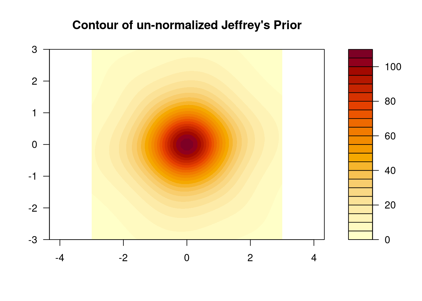
A somewhat reassuring image. The plot looks to be regular, but the distribution
is not elliptical, unless the weirdness in the tails is just a numerical error.
I don’t really believe that the prior has this “star” pattern, it’s more likely
either a plotting or computational problem.
After more experimentation and reflection, this seems to be neither a computational nor plotting artifact. In fact, the prior does have oblong tails due to the noise in the \(X\) matrix.
Sampling from the Posterior
To explore the posterior distribution we can use a Metropolis-Hastings algorithm. This might be the most general algorithm for generating posterior samples, but is also the most temperamental.
The (proportional) log-likelihood for Bernoulli logistic regression is,
\[ \ell(\boldsymbol{\beta} | X, y) \propto \sum_{i=1}^N \{ y_i \log \{ F(\boldsymbol{x}_i ^ \intercal \boldsymbol{\beta} ) \} \times (1 - y_i) \log \{ 1 - F(\boldsymbol{x}_i ^ \intercal \boldsymbol{\beta} ) \} \}, \]
which is much simpler to write in R code due to vectorization:
prop.to.loglike <- function(beta, X, y) {
  beta <- c(beta)
  sum(y * log(F(X %*% beta)) + (1 - y) * log(F(X %*% beta, lower.tail = FALSE)))
}
Metropolis-Hastings Sampler (Random walk version)
Choose a symmetric distribution, \(f\).
Let the Markov Chain have current state \(\theta_t\).
Generate proposal \(\xi = \theta_{t} + \epsilon\), where \(\epsilon \sim f\).
Define \(\rho = \min \{1, g(\xi) / g(\theta)\}\).
Accept the proposal with probability \(\rho\) (Set \(\theta_{t+1} = \xi\)). Otherwise, set \(\theta_{t+1} = \theta_t\).
Iterate (2.).
The outcome is a Markov Chain converging to the posterior. This is a decent solution for small models, but won’t scale well if the number of predictor variables is large.
In our case, \(g\) is the product of likelihood and prior, and we work on the log scale in an attempt to avoid numerical problems. The log-posterior is given by
\[ \log(\pi(\boldsymbol{\beta}|X,y)) \propto \log(L(\boldsymbol{\beta}|X,y)) + \log(\pi(\boldsymbol{\beta}|X)) , \]
so our MH algorithm is based on the ratio
\[ \frac{ g(\boldsymbol{\xi}) }{ g(\boldsymbol{\theta}) } = \exp \{ \log(L(\boldsymbol{\xi}|X,y)) + \log(\pi(\boldsymbol{\xi}|X)) - \log(L(\boldsymbol{\theta}|X,y)) - \log(\pi(\boldsymbol{\theta}|X)) \} \]
First, we need some data to try this out on. I just found some data on Google for a logistic regression that predicts the probability that a student is admitted to a school based on their gpa and class rank.
## I just found this on google
dat <- read.csv("https://stats.idre.ucla.edu/stat/data/binary.csv")

## Example bias reduction fit from brglm2 package (should be similar to our MH)
fit <- glm(admit ~ rank + gpa, binomial, dat, method = "brglmFit")

## Extract design matrix
X <- model.matrix(fit)

## Create response vector
y <- dat$admit
Finally, we can code up the M-H algorithm for logistic regression with a Jeffrey’s prior.
Here is the trick to make it run quickly: initialize the MC chain at the
coefficients of a frequentist model fit (I used brglm), and use the
variance-covariance matrix of the model fit for the variance of \(\epsilon\). This
is a good way to ensure a high acceptance ratio.
mh <- function(n, X, y, fit) {

  ## vector to store un-normalized log-posterior
  lp <- rep(NA, n)

  ## matrix to store the samples
  samps <- matrix(NA, n, ncol(X))
  colnames(samps) <- colnames(X)

  for (i in 1 : n) {

    ## Start the sampler at the brglm coefficients
    if (i == 1) samps[i, ] <- theta <- coef(fit)

    ## Generate a proposal. diag(diag(x)) extracts diagonal of x into vector then
    ## makes a diagonal matrix from it
    xi <- theta + rmvnorm(1, c(0, 0, 0), diag(diag(vcov(fit))))

    ## MH numerator
    log.num <- prop.to.loglike(xi, X, y) + prop.to.logprior(xi, X)

    ## MH denominator
    log.denom <- prop.to.loglike(theta, X, y) + prop.to.logprior(theta, X)

    ## Acceptance probability
    rho <- min(1, exp(log.num - log.denom))

    if (runif(1) < rho) {
      samps[i, ] <- theta <- xi
      lp[i] <- log.num
    }

    ## If not accepted, stick with the previous proposal
    else {
      samps[i, ] <- theta
      lp[i] <- log.denom
    }
  }
  cbind(samps, lp)
}
Run the MCMC sampler. I will take 10,000 samples. We don’t need to discard burn-in because we are smart about where we started the chain.
## Number of samples to take
n.samp <- 1e4

## Run the sampler, one chain, don't discard burn-in.
mc <- mh(n.samp, X, y, fit)
Diagnostics
Plot the MCMC draws. I find the pairs function the most convenient way to do
this. The first three panels are regression parameters, the final facet is the
log-posterior, which is somewhat less important.
## Plot the mc draws
pairs(mc)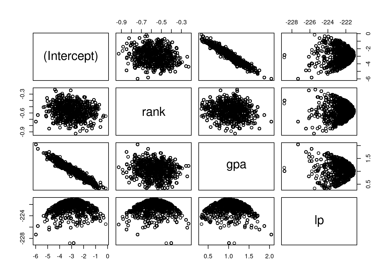
The acceptance rate appears to be low, but I find this changes a lot from run to run. Sometimes I get lucky, and the acceptance rate is in the 30% range.
nrow(unique(mc)) / nrow(mc) * 100 #percent units## [1] 6.12It’s also useful to look at a trace plot, and try to spot the ‘fuzzy caterpillars’
caterpillars <- melt(data.frame(mc[, 1 : 3]))

ggplot(caterpillars, aes(rep(1 : n.samp, 3), value)) +
  geom_line() +
  facet_grid(rows = vars(variable), scales = "free") +
  xlab("Index") +
  ggtitle("Trace Plot")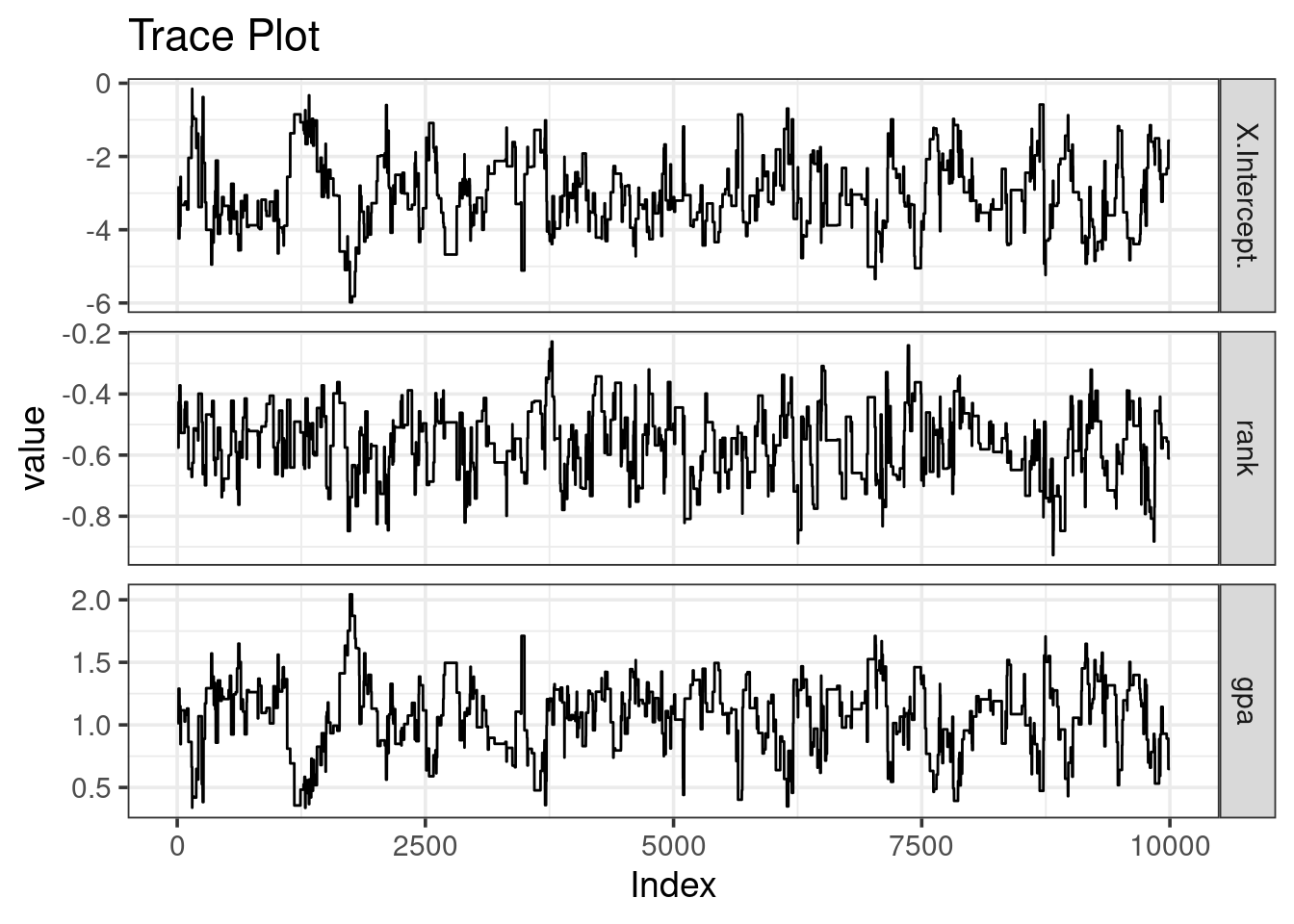
Our caterpillars are not fuzzy!
The chain mixing is… very poor, which we should have expected from the very low acceptance rate. If this was a more important problem, I might recommend thinning the chain.
Confirm the MH algorithm agrees with brglm
The posterior mode is the observation with the greatest log-posterior value. We saved the log-posterior during the MH algorithm, so we can easily pick off the mode.
mc[which.max(mc[, 4]), ] # Coefficients at mode of Bayesian model## (Intercept) rank gpa lp
## -2.8464717 -0.5752588 1.0136309 -221.0804054coef(fit) # Coefficients from brglm## (Intercept) rank gpa
## -2.8464717 -0.5752588 1.0136309The coefficients have perfect agreement. Success!
While it is nice to be able to recreate brglm from scratch, I don’t recommend
using the MH code. The MCMC performance is too variable. Better to stick with
the battle hardened R packages.
Except, lots of people will complain about this: If the data are perfectly separated, that means logistic regression is no good here. Better to move on than try to put a bandaid on this.↩
The latter has some very helpful vignettes on the R package page.↩
If we distinguish between binomial logistic regression and Bernoulli logistic regression, but there is rarely a need.↩