
How far can you take the nomogram?
A nomogram is an easy visual description of a fitted model. Nomogram creation is facilitated by the rms package in R. They are popular as a tool to give physicians, so that someone can estimate (say) the probability of hazardous side-effect without plugging numbers into an equation.
library(rms)Let’s take a previous data set, the college admission data from UCLA. From the data, one can model the probability of college admision using two variates, high school gpa, and class rank.
For simplicity, we can use logistic regression, but nomograms work for any binary data model (so probit regression or other special CDF regressions) and many general types of regressions models (OLS, Cox, and so on).
dat <- read.csv("https://stats.idre.ucla.edu/stat/data/binary.csv")
ddist <- datadist(dat)
options(datadist = "ddist")
Main effects model:
The nomogram for a main effects model is the simplest.
fit <- lrm(admit ~ gpa + rank, dat)
plot(nomogram(fit, fun = plogis, lp = FALSE))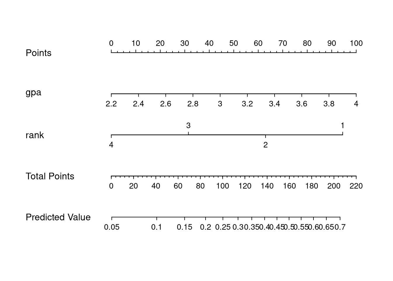
It takes a moment to get used to reading these charts, but the good way is to learn by example.
Suppose we have a student with a 4.0 GPA and a class rank of 1. Then the student is on the right hand side of nomogram. We look up the number of points associated with a 4.0 GPA (about 100 points) and a class rank of 1 (about 95 points) at the top line. The sum (about 195 points) is plugged into the second to last line. Then we take the prediction to be the value directly below 195 – about 65% in this case.
Interaction model with factors:
If we had an interaction, the nomogram would be split into more pieces, but the idea is the same.
fit <- lrm(admit ~ gpa * rank, dat)
plot(nomogram(fit, fun = plogis, lp = FALSE))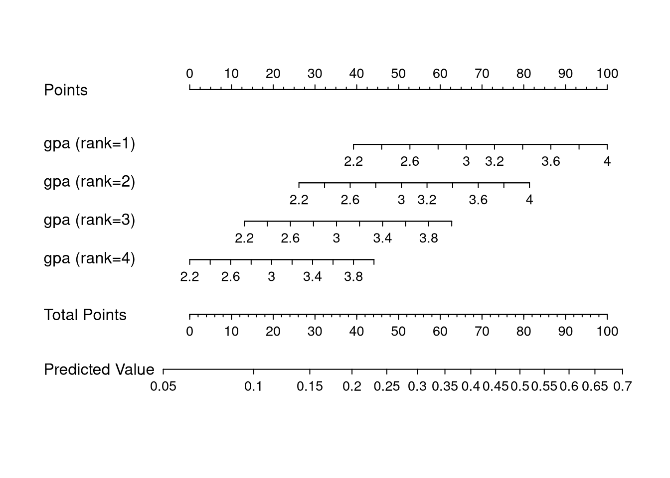
Restricted cubic spline model
If we choose to model with some transformations, the scales are transformed accordingly, but the usage is the same
fit <- lrm(admit ~ rcs(gpa, 4) + rank, dat)
plot(nomogram(fit, fun = plogis, lp = FALSE))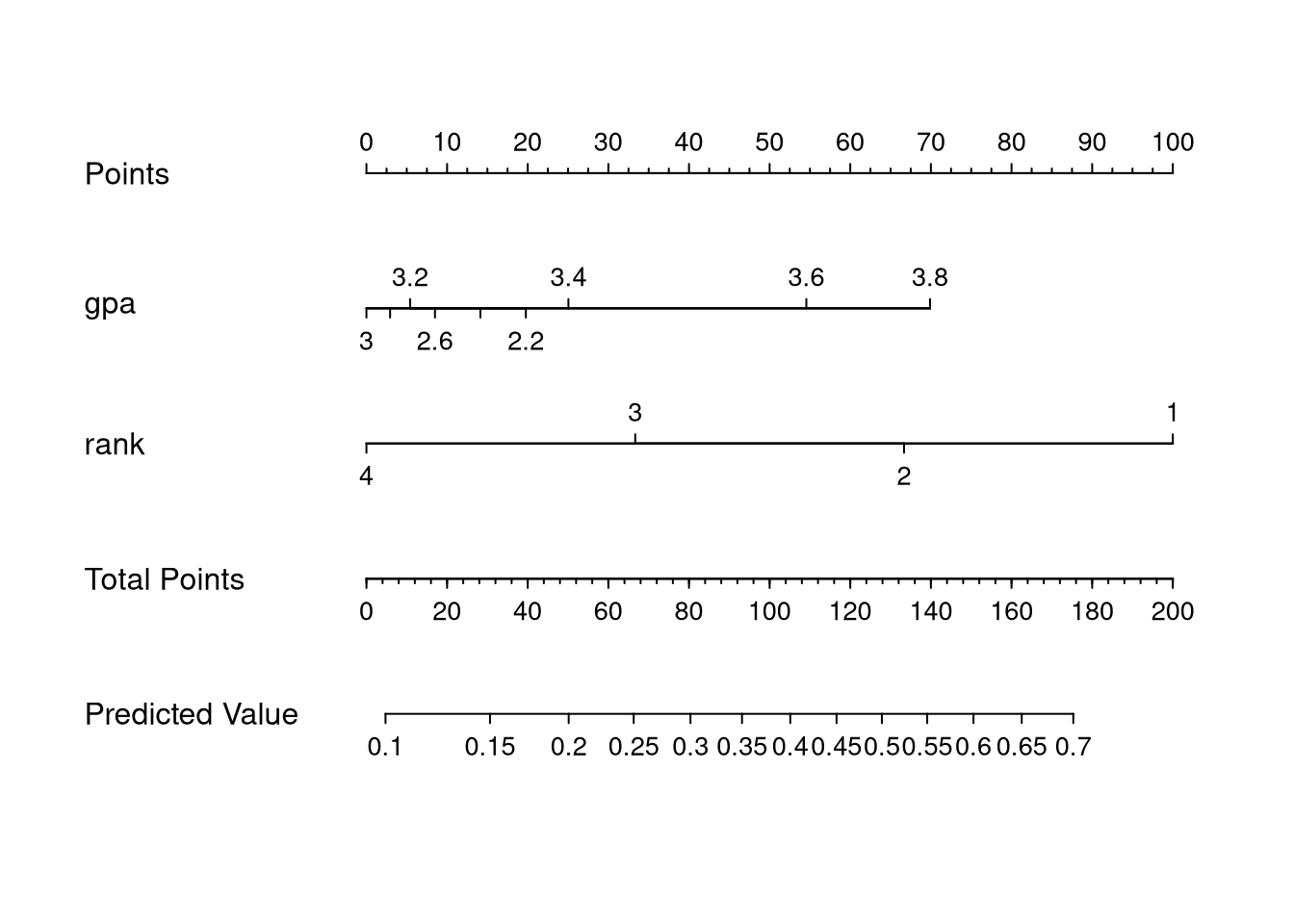
RCS model with interaction
Transformations can be combined with interactions too:
fit <- lrm(admit ~ rcs(gpa, 4) * rank, dat)
plot(nomogram(fit, fun = plogis, lp = FALSE))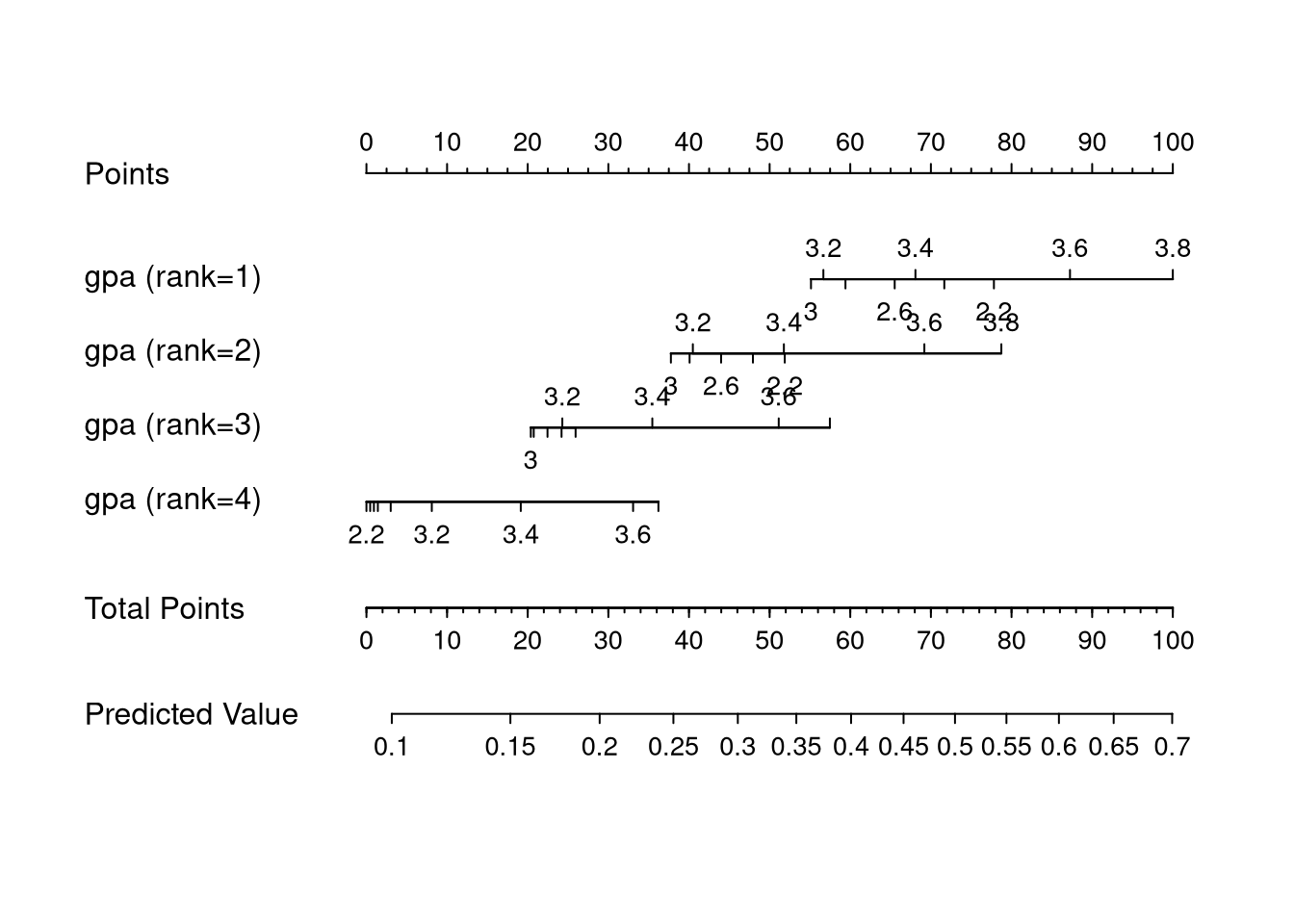
Interaction between two continuous variables
If we interact two continuous variables, we have to choose cutpoints in order to draw the nomogram. It is not very clean, but possible.
## Create a new vector
dat$x <- rnorm(nrow(dat))
ddist <- datadist(dat)
fit <- lrm(admit ~ rcs(gpa, 4) * x, dat)
plot(nomogram(fit,
  fun = plogis, lp = FALSE,
  interact = list(x = seq(-3, 3, 2))))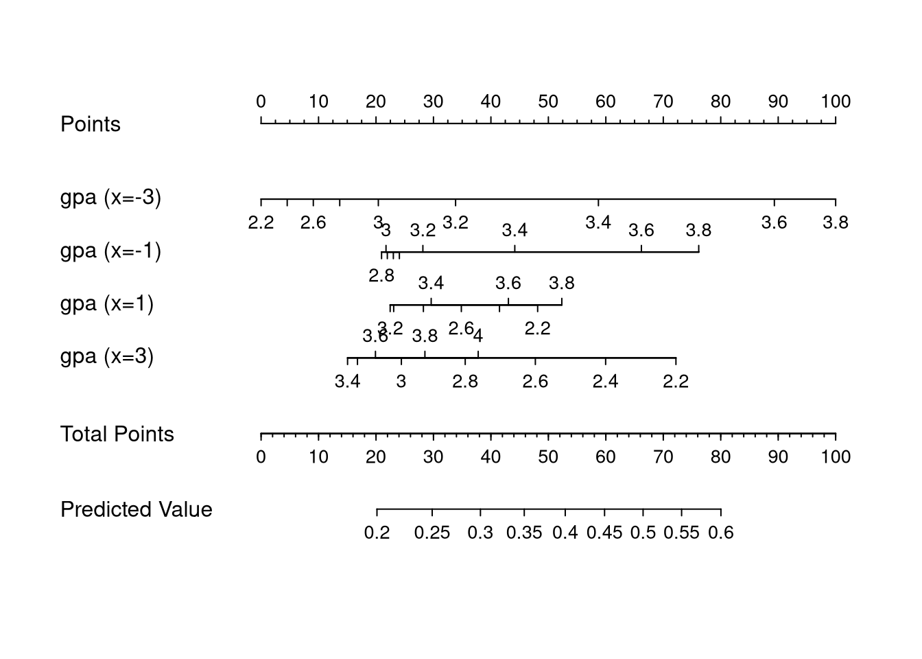
Nomograms are very useful tool for non-statisticians to make predictions without a computer, and they are useful for statisticians to understand what a complicated model “looks like”. We cannot simply graph a model with 6 variables, but we can easily make a nomogram.