
Using Bayesian statistics at work, sometimes there is a bias towards conjugate priors. Conjugate priors are great due to their computational easiness and pedagogical utility. Specifically, you don’t even need to use a Markov chain sampler if the likelihood has a conjugate prior, you just need to look up the formula for your posterior, and update the parameters according to the prior/likelihood combo you are working with.
But, sometimes we need to go a bit further, because the solutions we are conceptualizing don’t really fit into the conjugate prior framework. I was looking at a problem recently that benefited from a prior distribution that could be written as the product of two Gamma distributions. The rationale was that the second Gamma variable could be used as kind of decrement on the first Gamma variable, and due to the inputs to the problem, it was useful to leave the first Gamma variable alone. The complete set up for the problem looked like this:
\[ \theta \sim \textrm{Gamma}(\alpha, \beta) \times \textrm{Gamma}(\alpha_2, \beta_2) \]
\[ c|\theta \sim \textrm{Exponential}(\theta) \]
In the Bayesian formulation, the objective is to characterize the distribution of \(\theta|c\). If the second Gamma distribution had been omitted from the prior, we would have a perfectly fine conjugate prior situation, but it’s presence means that we must reach for a more advanced technique, such as a Markov chain sampler. My preference is to use a random walk Metropolis Hasting sampler, which we have previously employed on this blog.
The only wrinkle here is that one may sample on the log-scale to use the random walk version of the Metropolis sampler, which introduces the requisite Jacobian in the posterior. If you prefer to use the general Metropolis Hasting algorithm, you don’t need to convert to the log-scale.
## Set required params in prior/likelihood
alpha <- 10
beta <- 10
alpha2 <- 10
beta2 <- 10
c <- 1

## Define a function that outputs proportional to the posterior
prop.to.post <- function(log.lambda) {
  dexp(x = c, rate = exp(log.lambda)) *
    dgamma(exp(log.lambda), shape = alpha, scale = beta) *
    dgamma(exp(log.lambda), shape = alpha2, scale = beta2) *
    exp(log.lambda) # jacobian

}

nsim <- 10000
samps <- numeric(nsim)

## Run the sampler
for (i in 1:nsim) {
  if (i == 1) samps[i] <- theta <- 1
  xi <- theta + rnorm(1)
  rho <- min(1, prop.to.post(xi) / prop.to.post(theta))
  if (runif(1) < rho) {
    samps[i] <- theta <- xi
  } else {
    samps[i] <- theta
  }
}

post.samps <- exp(samps)
hist(post.samps, breaks = 50)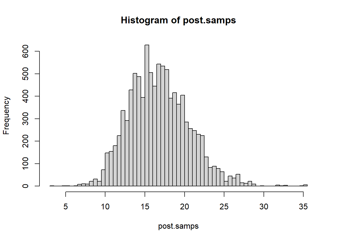
You might have noticed one area where we could have made the sampler a bit more computationally robust. We multiplied densities together, and whenever we do something like that, it is always better to work with the sums of log densities.