
Introduction
Factor importance popped up on Cross Validated again today, with the question being how one can determine which predictor is most meaningful, and how to order the predictors by meaningfulness.
Lately, I’ve not had the gusto to fully answer questions, so I just commented that I would use analysis of variance to determine the factors that are meaningful in the regression model. I further commented that I would use the statistic \(\chi^2 - df\) to assess or order the meaningfulness, but I preempted some criticism by stating that this is my preference, and that the choice is subjective.
I have written in the past about ANOVA pie charts for the purpose of decomposing variance explained, but since the publication of that post, my thinking on variable importance has evolved beyond the confines of base-R, and I now think that the using sums of squares approach is too limiting for most of the problems that I typically face, as this requires one to use the dreaded Type I SS in addition to the correctly specified model to actually determine factor importance.
The advantage of the \(\chi^2 - df\) approach is that ANOVA can be penalized by the complexity of the factor. This is very much needed when some variables have a high number of degrees of freedom, because under the null hypothesis, the \(\chi^2\) ANOVA statistic is equal to the df of the factor. Without penalization, a meaningless, but complex factor can appear as relevant as an important, but simple, factor.
The choice of factor importance statistic really is subjective because the statistical question is under-specified: There is no parameter that one can estimate that actually corresponds to factor importance1.
The anova function in the rms package is just the ticket for calculating penalized ANOVAs. Let’s take a fake data example:
library(lme4)
library(rms)
Data and Model
Let’s take the cake dataset from lme4 to demonstrate the ANOVA concepts from rms. The help page for the dataset gives the following description of the factors:
Data on the breakage angle of chocolate cakes made with three different recipes and baked at six different temperatures. This is a split-plot design with the recipes being whole-units and the different temperatures being applied to sub-units (within replicates). The experimental notes suggest that the replicate numbering represents temporal ordering.
A data frame with 270 observations on the following 5 variables.
replicate: a factor with levels 1 to 15
recipe: a factor with levels A, B and C
temperature: an ordered factor with levels 175 < 185 < 195 < 205 < 215 < 225
angle: a numeric vector giving the angle at which the cake broke.
temp: numeric value of the baking temperature (degrees F).
The suggested (full) model from the examples section is angle ~ recipe * temperature + (1|recipe:replicate), but I will avoid the random effects for now.
A simple linear model with analysis of variance can be applied:
form <- angle ~ recipe * temperature + recipe * replicate
fit <- ols(form, cake)
cake_aov <- anova(fit) # note: anova.rms, not anova.lm
An ANOVA table is calculated2:
options(prType='html')
html(cake_aov)
Analysis of Variance for angle | |||||
| d.f. | Partial SS | MS | F | P | |
|---|---|---|---|---|---|
| recipe (Factor+Higher Order Factors) | 40 | 1539.5333 | 38.48833 | 1.88 | 0.0024 |
| All Interactions | 38 | 1404.4444 | 36.95906 | 1.81 | 0.0049 |
| temperature (Factor+Higher Order Factors) | 15 | 2306.2778 | 153.75185 | 7.51 | <0.0001 |
| All Interactions | 10 | 205.9778 | 20.59778 | 1.01 | 0.4393 |
| Nonlinear (Factor+Higher Order Factors) | 12 | 337.8311 | 28.15259 | 1.38 | 0.1796 |
| replicate (Factor+Higher Order Factors) | 42 | 11402.7111 | 271.49312 | 13.26 | <0.0001 |
| All Interactions | 28 | 1198.4667 | 42.80238 | 2.09 | 0.0018 |
| recipe × temperature (Factor+Higher Order Factors) | 10 | 205.9778 | 20.59778 | 1.01 | 0.4393 |
| Nonlinear | 8 | 204.2362 | 25.52952 | 1.25 | 0.2732 |
| Nonlinear Interaction : f(A,B) vs. AB | 8 | 204.2362 | 25.52952 | 1.25 | 0.2732 |
| recipe × replicate (Factor+Higher Order Factors) | 28 | 1198.4667 | 42.80238 | 2.09 | 0.0018 |
| TOTAL NONLINEAR | 12 | 337.8311 | 28.15259 | 1.38 | 0.1796 |
| TOTAL INTERACTION | 38 | 1404.4444 | 36.95906 | 1.81 | 0.0049 |
| TOTAL NONLINEAR + INTERACTION | 42 | 1538.0394 | 36.61998 | 1.79 | 0.0042 |
| REGRESSION | 59 | 13844.0778 | 234.64539 | 11.46 | <0.0001 |
| ERROR | 210 | 4298.8889 | 20.47090 | ||
In total, the regression is estimated with 59 model degrees of freedom and 210 error degrees of freedom. Of course, a random effects model would be more efficient with the data, but nevermind that bit. While the table is fairly nice, a graph is better:
The recommended ANOVA table
plot(cake_aov,
     main = expression(paste(chi^2 - df, " type ANOVA for cake data")))
Explanation
The \(\chi^2\) statistic is the partial \(F\) statistic for each model term, multiplied by the associated degrees of freedom. The partial-F statistic is
\[ F = \frac{\frac{SSE_{Reduced Model} - SSE_{Full Model}}{d}} {\frac{SSE_{Full Model}}{n-k}}. \]
Where SSE is the sum of squared errors for either the full model (the one we want to determine the important factors of) or the reduced model (full model minus one factor we interrogate for relevance). \(d\) is the df of the tested factor, so the \(\chi^2\) statistic is just \(d \times F\). The statistic has expected value \(d\). \(n-k\) is the degrees of freedom of the error term.
Another way to write this ANOVA statistic is \(d \times F - d\).
Many factors are significant, but the recipe by temperature interaction is not. The driving factor might be replicate, which means that most of the model variance could be attributable to differences between replicates.
And what about the other styles of ANOVA tables? Of course, we can compute them with rms as well.
The Other \(\chi^2\) ANOVA tables
plot(cake_aov,
     what = "chisq",
     main = expression(paste(chi^2, " type ANOVA for cake data")))
Explanation
Same as above, except we calculate \(d \times F\) rather than \(d \times F - d\). So this is the same statistic without penalization.
plot(cake_aov,
     what = "aic",
     main = paste("AIC type ANOVA for cake data"))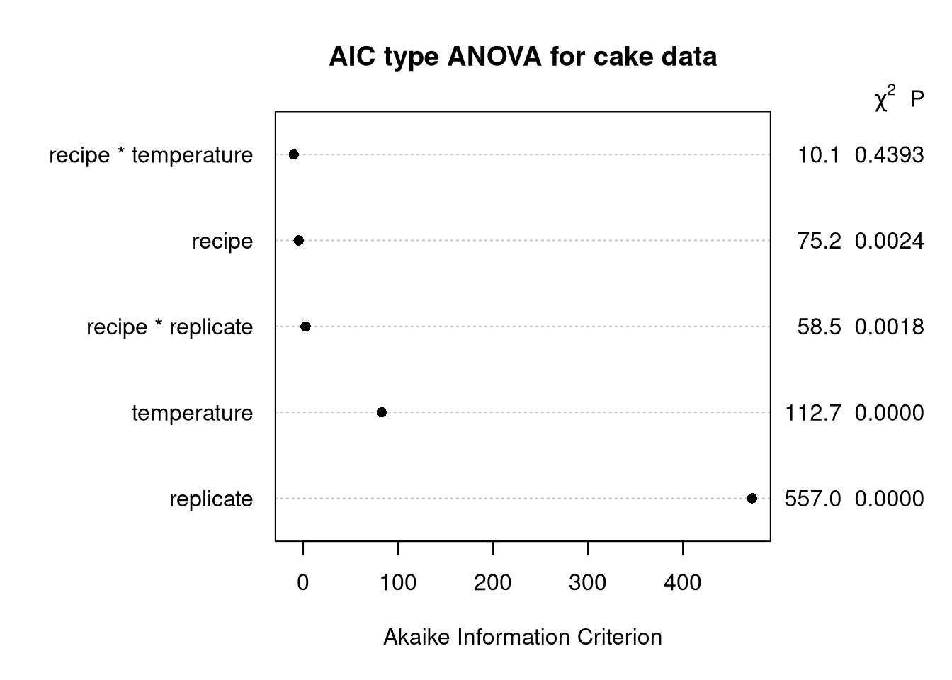
Explanation
Same as the penalized \(\chi^2\) ANOVA, but we calculate \(d \times F - 2d\) to draw the table.
I find this one the most curious because, while I’m quite aware that model AIC is \(2k - 2 * \log (\hat L)\), seeing some version of AIC used for ANOVA is totally new.
plot(cake_aov,
     what = "proportion chisq",
     main = expression(paste("ANOVA table based on proportional ", chi^2, " statistic")))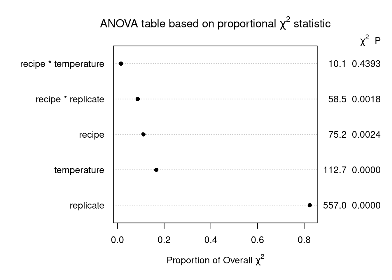
Explanation
Define the model \(\chi^2\) statistic as the model’s F statistic times the model degrees of freedom. For this model, the F stat is \(11.46\) and the model df is \(59\). Call this model \(\chi^2\) statistic \(M\). Then each row of the ANOVA table is \(dF/M\).
plot(cake_aov,
     what = "P",
     main = "ANOVA table based on p-values")
Explanation
ANOVA table using the \(p\)-value from each partial \(F\) test. In theory, a smaller \(p\)-value equates to a more meaningful factor. In this case, the table isn’t too informative, many \(p\)-values are near zero, so it’s hard to interpret. A log scale is recommended for this plot to better differentiate between factor effects, but we will move on.
ANOVA tables based on \(R^2\)
The following are based on the Type III ANOVA partial Sums of Squares calculated by rms::anova.
plot(cake_aov,
     what = "partial R2",
     main = expression(paste("ANOVA table based on partial ", R^2, "statistic")))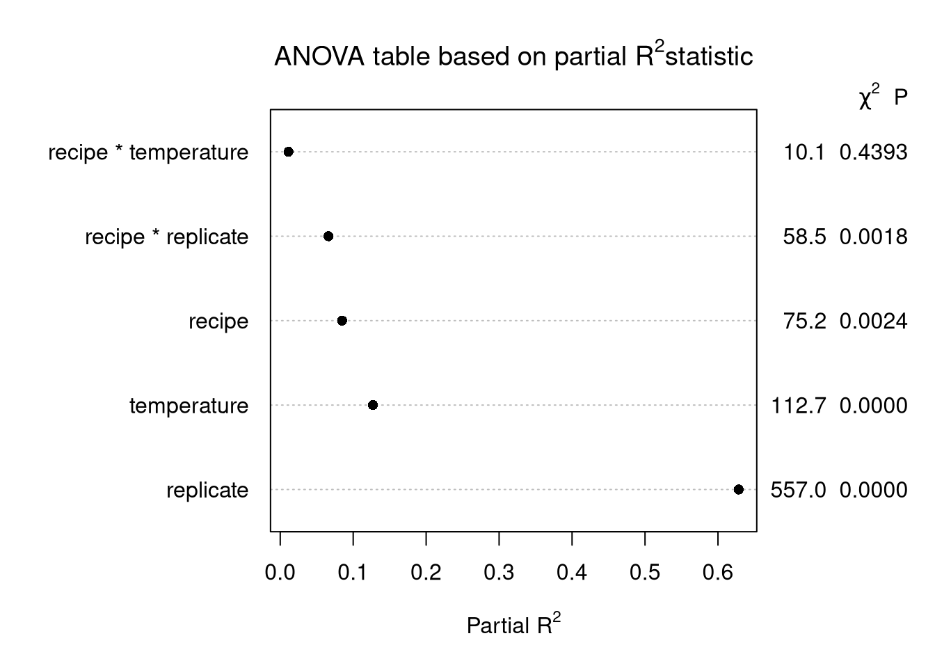
Explanation
Use \(SST = SSR + SSE\), the usual ANOVA decomposition, and for each factor calculate partial SS divided by SST.
plot(cake_aov,
     what = "remaining R2",
     main = expression(paste("ANOVA table based on remaining ", R^2)))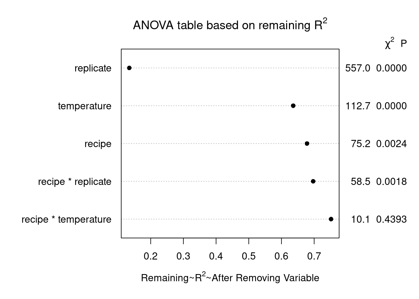
Explanation
Similar to the above, except draw the plot using \(\frac{\mathrm{SSR} - \mathrm{Partial SS}}{\mathrm{SST}}\).
plot(cake_aov,
     what = "proportion R2",
     main = expression(paste("ANOVA table based on proportional ", R^2)))
Explanation
Similar to the above, except draw the plot using \(\frac{\mathrm{Partial SS}}{\mathrm{SSR}}\).