
We just discussed the different ANOVA methods for calculating factor relevance. While there are a lot of fairly decent ways to tease out factor relevance1, the methods are also subject to error. Unfortunately the random noise that is inherent to factor importance methods is almost always missing from the analysis.
In this post, I want to demonstrate methods that could be useful for displaying the uncertainty in factor relevance metrics. Let’s return to the cake data that we used in the previous post.
library(lme4) # for data set
library(ggplot2); theme_set(theme_bw(base_size = 14))
library(forcats)
library(rms) # for anova method
library(data.table)
form <- angle ~ recipe * temperature + recipe * replicate
fit <- ols(form, cake)
cake_aov <- anova(fit)
plot(cake_aov)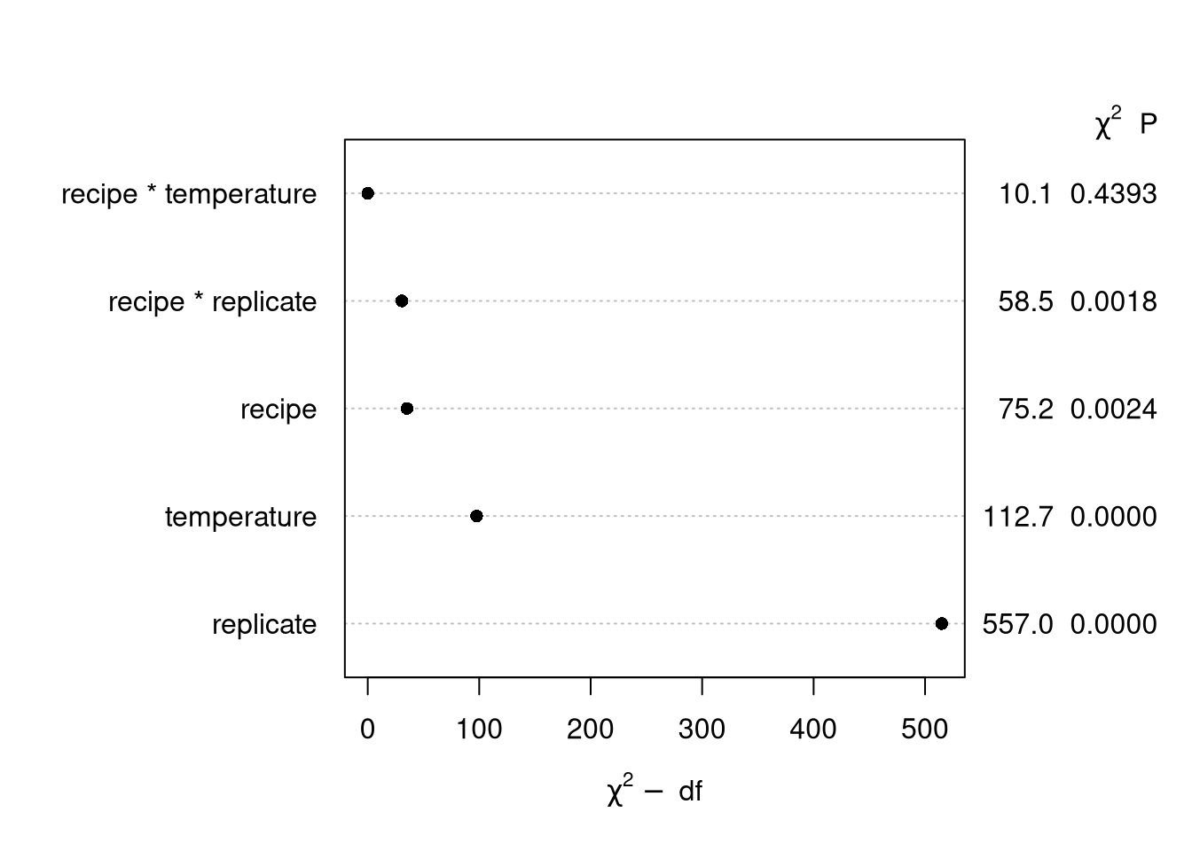
“Poor man’s posterior”
I recommend using a bootstrap procedure for the sake of simplicity. For regression problems, we must choose between one of two2 boostrap procedures for the model.
Resample the data. Use this procedure for “found data”. Basically, this is the ordinary bootstrap
Resample the residuals. Use this procedure for experimental data. Basically, we will resample the residuals, then produce a new resampled outcome. This is a good procedure for experiments because it does not muck with the experimental design: all bootstrap replicates have the same design.
Here is the basic residual bootstrap for our data.3
aovs <- list()
B <- 1000
res <- residuals(fit)
linpred <- predict(fit)
formb <- y_b ~ recipe * temperature + recipe * replicate
var <- copy(cake)
cake_b <- setDT(var)

for (i in 1:B) {
  res_b <- sample(res, replace = TRUE)
  y_b <- linpred + res_b
  cake_b$y_b <- y_b
  fit_b <- ols(formb, cake_b)
  aovs[[i]] <- anova(fit_b)
}
Now, for each of the bootstrap ANOVAs, we need to calculate the plot statistics, penalized \(\chi^2\) values. These are not readily available, so I have to loop over the list calculate them myself.
chisqps <- list()
ind <- c(1, 3, 6, 8, 11) # indices of factor effects

for (i in 1:B) {
  dof <- aovs[[i]][, "d.f."]
  F <- aovs[[i]][, "F"]
  chisqp <- F * dof - dof
  chisqps[[i]] <- data.frame(stat = chisqp[ind],
                             factor = names(chisqp)[ind])
}

## combine simulation data
bstats <- rbindlist(chisqps)

## Remove unslightly information from factor levels
bstats[, factor := gsub("\\(.+\\)", "", factor)]
bstats[, factor := fct_reorder(factor, stat, .desc = TRUE)]

## ## I also need to collect the anova statistics from the original model fit as well:
dof <- cake_aov[, "d.f."]
F <- cake_aov[, "F"]
chisqp <- F * dof - dof
chisqp_orig <- chisqp[ind]

orig_df <- data.table(factor = names(chisqp_orig),
                      stat = chisqp_orig)

orig_df[, factor := gsub("\\(.+\\)", "", factor)]
orig_df[, factor := fct_reorder(factor, stat, .desc = TRUE)]
And we can plot the original ANOVA statistics with their bootstrap replicates:
ggplot(bstats, aes(x = factor, y = stat)) +
  coord_flip() +
  geom_violin(fill = "gray") +
  xlab("") +
  ylab(expression(chi ^ 2 - d.f.)) +
  scale_color_manual(values = c("Original" = "black")) +
  geom_point(aes(x = factor, y = stat, color = "Original"), orig_df, size = 2) +
  theme(legend.position = "bottom")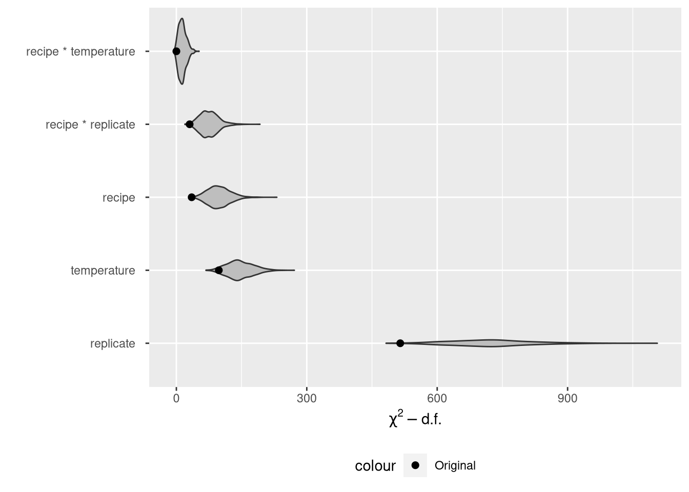
Two comments on this plot.
It is very hard to tell the difference between the middle three factors now that we’ve added the violin plots to the point estimates. There is real variability in the \(\chi^2\) stats.
The violin plots show that the model \(\chi^2\) statistics don’t line up well with the bootstrap replicates at all, implying considerable bias in the original statistics. However, the original statistics are not biased, since there’s no population parameter that corresponds to a \(\chi^2\) statistic. This makes the whole endeavor look a bit pointless.
Is there a better to show the noise in an ANOVA? Bayesians have a easy way of doing this. See here.